How to Sort Columns in Excel Without Mixing Data (6 Methods)

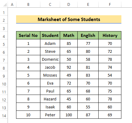
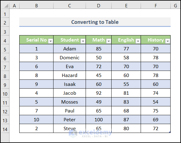
Dataset Overview

Suppose you have a basic table containing the names of students and their respective scores in three courses. In this scenario, we’ll explore how to sort columns without disrupting the data. Keep in mind that the example data provided here is simple; in real-world cases, you might encounter larger and more complex datasets.

Excel offers built-in tools for sorting data. Let’s walk through the process:

• Select the Column to Sort:
  • Choose the column you want to sort. For instance, let’s select the “Student Name” column and sort the names alphabetically (A to Z).
  • Navigate to the Data tab, where you’ll find the Sort & Filter option. Click on it to reveal several sorting options.

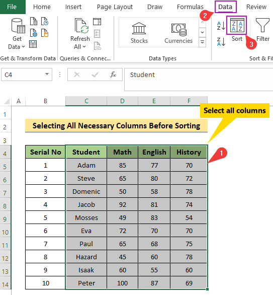
Method 1 – Select All Necessary Columns Before Sorting

• Go back to the initial data state.
• Follow these steps:
  • Select all the columns you want to include in the sort (except the “Serial No.” column, which should remain unchanged).
• Click the Sort option from the Data tab.

• A dialog box will appear, allowing you to choose your sorting preferences.

• Ensure that you check the My data has headers option.
• Since we’ve selected four columns, we can sort by any of them.
• Choose the Student Name column, sort by cell values, and set the order to A to Z.
• You can adjust these settings using the drop-down icons.

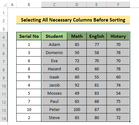
• After sorting, you’ll find the names in alphabetical order, and the corresponding scores will remain intact.

Method 2 – Using the ‘Expand the Selection’ Option

• Excel provides a warning before sorting, which is helpful.
• Follow these steps:
  • Select any column (e.g., Student Name) and explore the Sort & Filter section in the Data tab.
  • Choose the A to Z sorting option.
  • If you don’t select the entire table, Excel will display a warning.
  • You have two options:
    • “Continue with the current selection” (filters only the selected cells).
    • “Expand the selection” (counts all columns in the table).

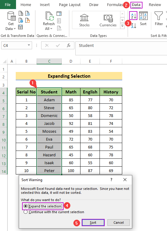
• We recommend using Expand the selection.
• Click Sort.

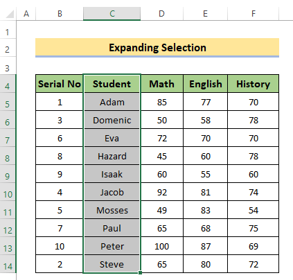
• The names will be sorted alphabetically, and other values will adjust accordingly.

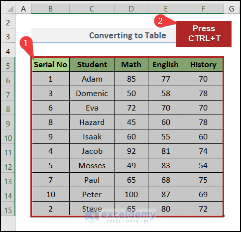
Method 3 – Converting to a Table

• Convert a normal data range into a table and then apply sorting.
• Follow these steps:
  • Select cells in the B4:F14 range (your data).
  • Press CTRL + T on your keyboard.

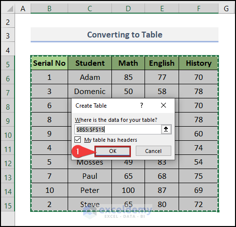
• The Create Table dialog box will appear; click OK.

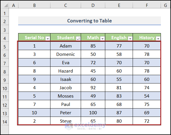
• Your data range is now a table.

• Select cells in the Student column.
• Go to the Data tab and click Sort A to Z.

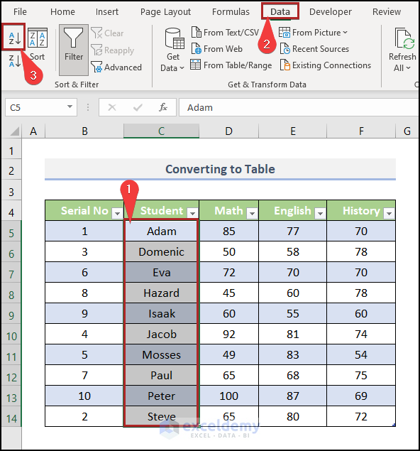
• The entire dataset will be sorted along with the Student column.

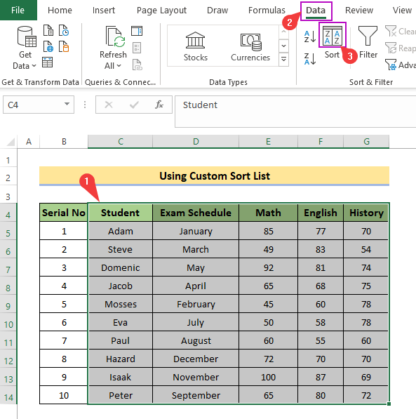
Method 4 – Creating a Custom Sort List to Prevent Mixing Data

You have the flexibility to sort data according to your preferences in Excel. The custom sorting feature can assist you with this task. Let’s consider an example where we’ve slightly modified our data:

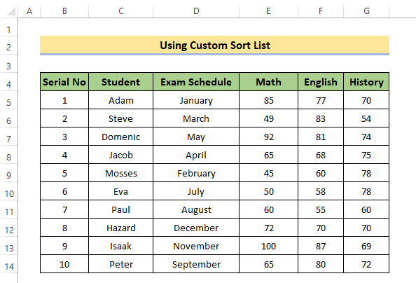
1. We’ve added a new column that indicates the month when students appeared for their respective exams.
2. Our goal is to sort the data without altering the existing serial numbers (which are already in sequence).

Steps:

• Select the Sort option from the Sort & Filter menu.

• A dialog box will appear.

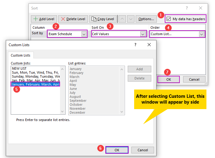
• Under Order, click the drop-down icon, and you’ll find an option called Custom List. Select it.
• Another dialog box, the Custom Lists dialog, will appear.
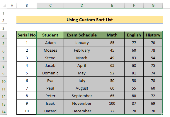
• Excel provides predefined lists for your convenience. In our case, we’ve chosen the months (from January to December). You can select a list that suits your needs.
• Specifically, we’ve sorted the Exam Schedule column based on the globally sequential months.

Read More: Sort Multiple Columns in Excel Independently of Each Other

Method 5 – Using the SORT Function in Excel

If you’re using Excel 365, you can take advantage of the SORT function. This function sorts the contents of a range or array in either ascending or descending order.

Steps:

• Enter the following formula in Excel:

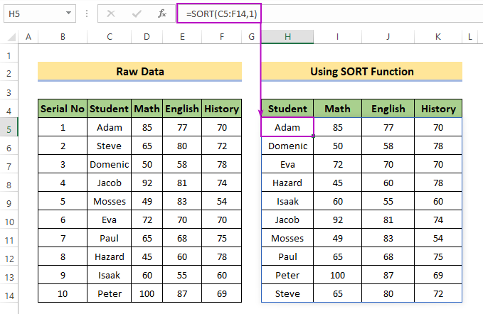
• We’ve applied this formula to the range from the Student Name column to the History column.
• Since we wanted to sort by name (which is the first column in the range), we inserted 1 as the sort_index.
• The data is now sorted alphabetically by names.

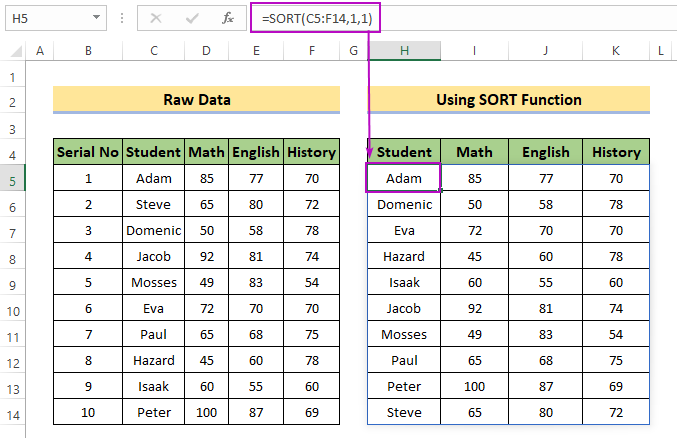
• For ascending order, you can insert 1 in the sort_order field:

• To sort in descending order, use -1 instead of 1 in the sort_order field:

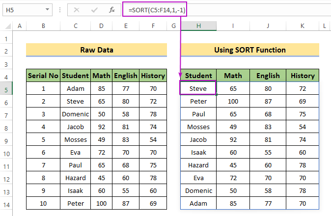
Method 6 – Sort Columns Without Mixing Data Using the SORTBY Function in Excel

The SORTBY function is closely related to the previously discussed SORT function. It sorts the contents of a range or array based on values from another range or array.

Steps:

• Apply the following formula in a desired cell:

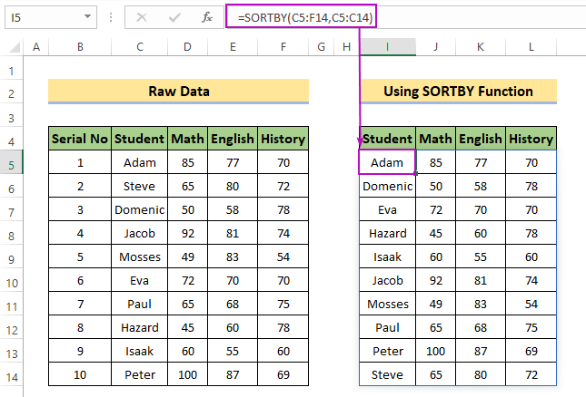
• • In this case, we’ve selected the array (range) from the Student Name column to the History column.
  • Our by_array was the Student Name column.
  • Unlike SORT, which uses column numbers, SORTBY allows sorting based on an array (column) directly.

• Let’s change the by_array.

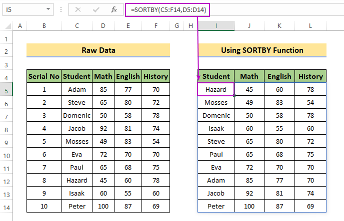
• • Now we’ve selected the Math column as our by_array.
  • The Math column has been sorted in ascending order, and the other column values adjusted accordingly.

Download Practice Workbook

You can download the practice workbook from here:

Related Articles

• How to Sort Two Columns in Excel to Match
• How to Sort Alphabetically in Excel with Multiple Columns

<< Go Back to Sort Columns in Excel | Sort in Excel | Learn Excel