Wouldn’t it be great to have the Titles at the top of every page when printing in Excel? With this in mind, this article demonstrates how to set multiple rows as Print Titles in Excel.
How to Set Multiple Rows as Print Titles in Excel: 4 Simple Ways
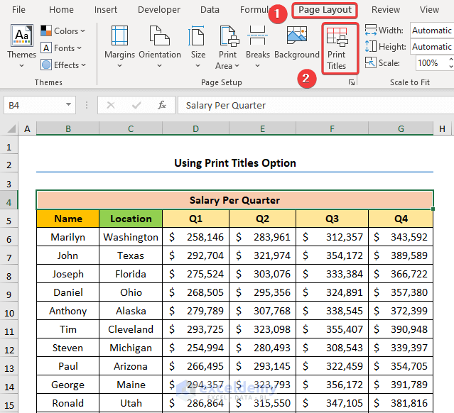
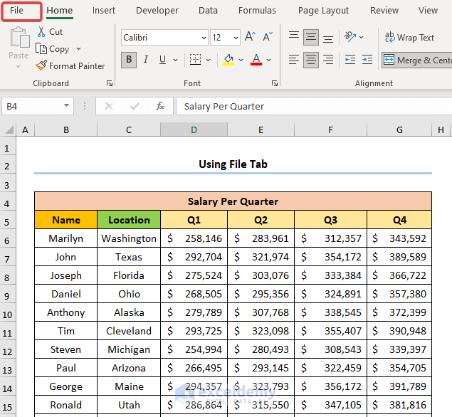
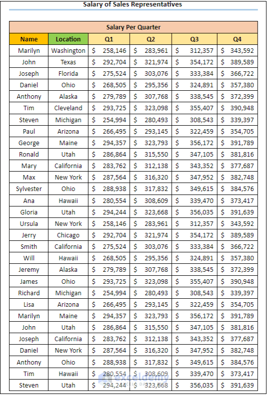
Let’s say, we have the Quarterly Salary of the Sales Representatives. Here, we want to print the headers’ Names, Locations, and Quarterly Salaries at the top of every page. So, without further delay, let’s see the methods one by one.


We have used Microsoft Excel 365 version here, you can use any other versions according to your convenience.
Method-1: Using Print Titles Option to Set Multiple Rows as Print Titles
For our first method, we’ll use the Print Titles option to print the headers at the top of each page.
Steps:
- Firstly, go to the Page Layout tab >> click the Print Titles option in the Page Setup group.
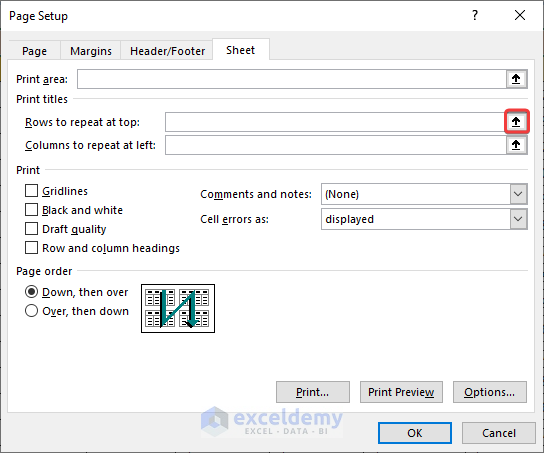
After completing this step, the Page Setup wizard appears.
- Next, click the arrow next to the Rows to repeat at top box.
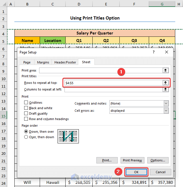
- Then, hold the CTRL key on your keyboard and select the header rows. In this case, we chose the $4:$5 rows as the headers.
- After this, press the OK button.
- Now, use the CTRL + P shortcut to open the Print option.
- Following this, click the arrow at the bottom to go to the next page.
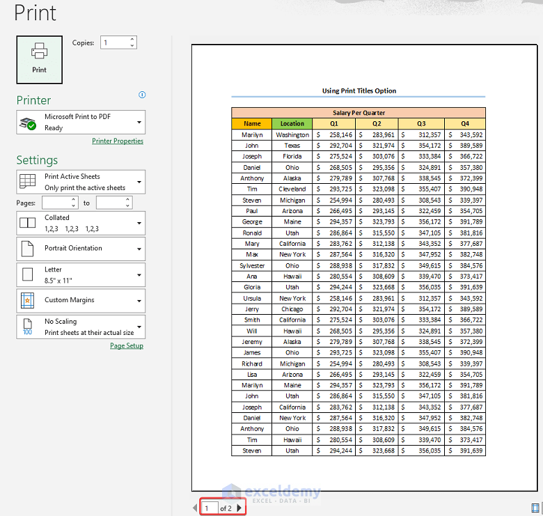
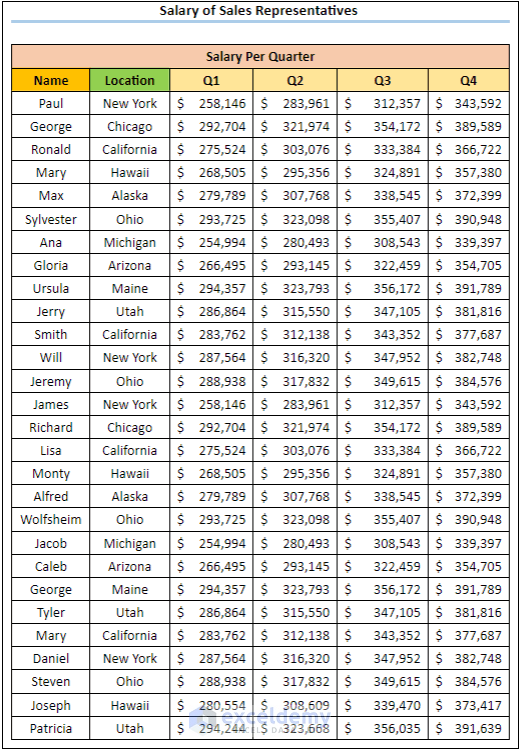
The preview for the second page should look like the image shown below.
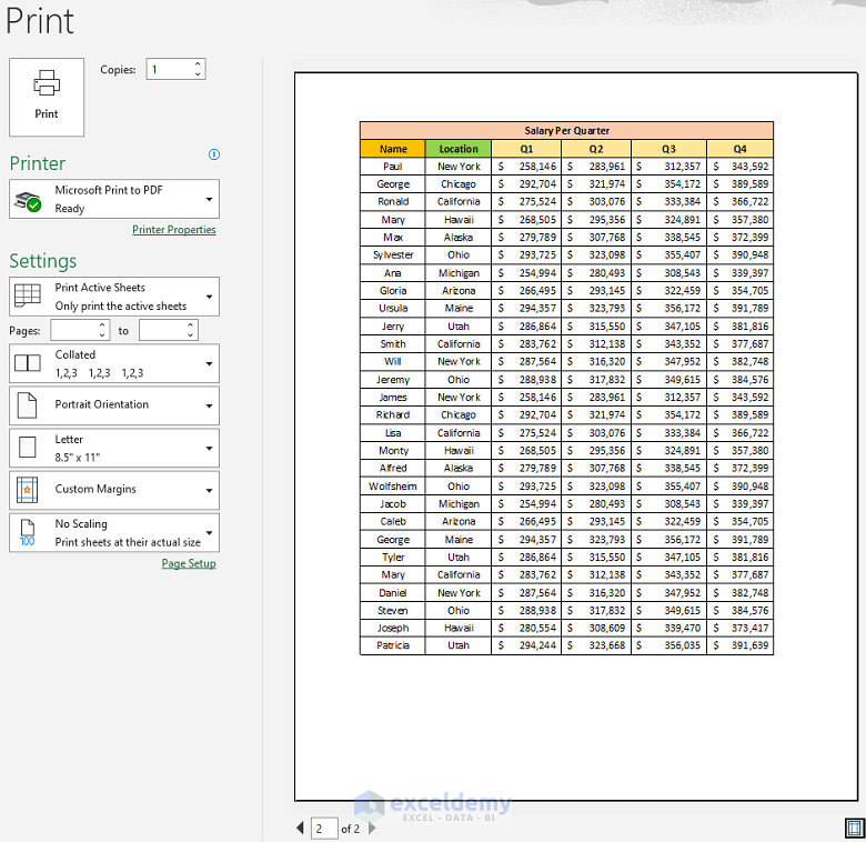
That’s it you’ve placed the headers at the top of every page. It’s that simple!
Read More: How to Set a Row as Print Titles in Excel
Method-2: Applying Keyboard Shortcut
Now, I know what you’re thinking. Are there any shortcut keys? Lucky you! There are shortcut keys for setting Print Titles. And our second method describes just that.
Steps:
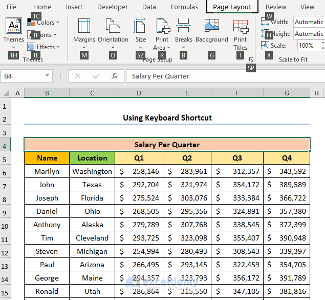
- Firstly, press the ALT key on your keyboard followed by P.
The Ribbon at the top should look like the picture shown below.
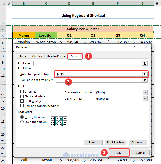
- Afterward, press S and then P on the keyboard. In an instant, the Page Setup dialog box pops up.
- Next, click the Sheet tab >> select the cell reference of the header rows ($4:$5) >> click on OK.
- Then, press the CTRL + P keys to go to the Print option.
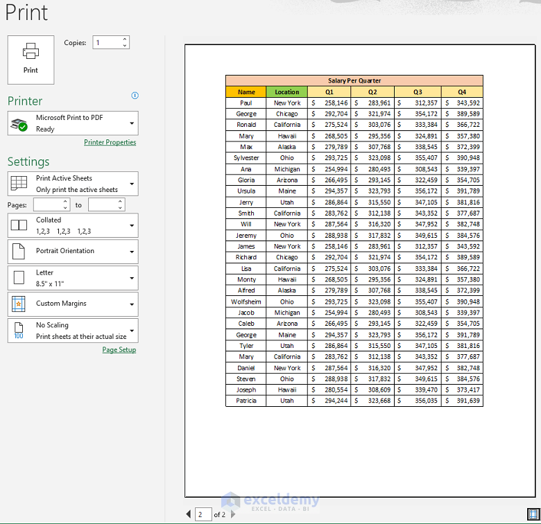
- Lastly, use the arrow button to examine the preview pages.

Finally, you’ll see the results as shown in the screenshot below.
Read More: Print Titles in Excel Is Disabled, How to Enable It?
Method-3: Set Multiple Rows as Print Titles in Excel from File Tab
For our third method, we’ll utilize the File tab to insert Print Titles. So, let’s see it in action.
Steps:
- Firstly, navigate to the File tab at the top-left corner of the Ribbon.
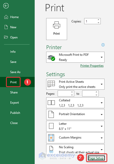
- Next, select the Print option >> then, click on the Page Setup button.
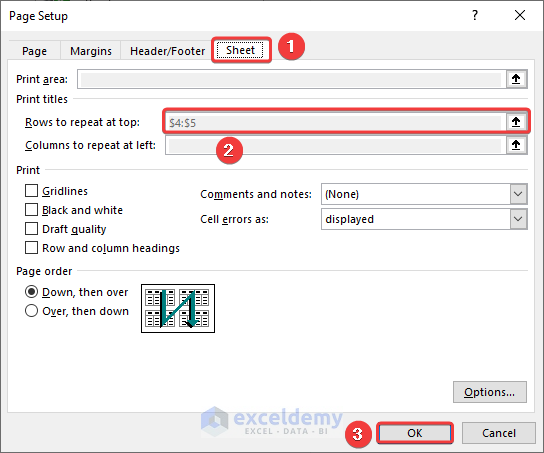
- Now, in the Page Setup wizard, move to the Sheet tab >> enter the reference $4:$5 for the titles >> click the OK button.
- Lastly, check the preview pages using the arrow key at the bottom.
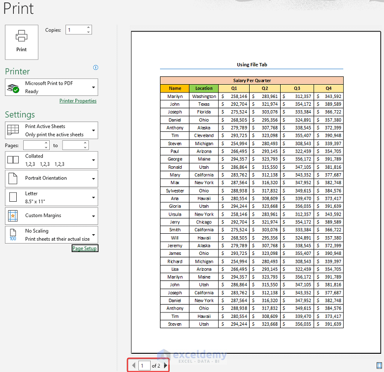
The second page of the worksheet looks like the image shown below.
Read More: [Fixed!] Print Titles Must Be Contiguous and Complete Rows or Columns
Method-4: Utilizing Freeze Pane Option to Set Multiple Rows as Print Titles in Excel
Excel’s Freeze Panes option allows us to see the column headers even if we scroll down. In this method, we’ll apply the Freeze Panes feature to insert the Print Titles at the top of each page when printing. So, follow these simple steps.
Steps:
- Firstly, select the row before which you want to freeze. In this case, Row 6 is selected.
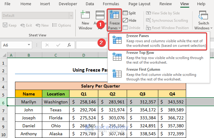
- Secondly, move to the View tab >> click the Freeze Panes drop-down in the Window section.
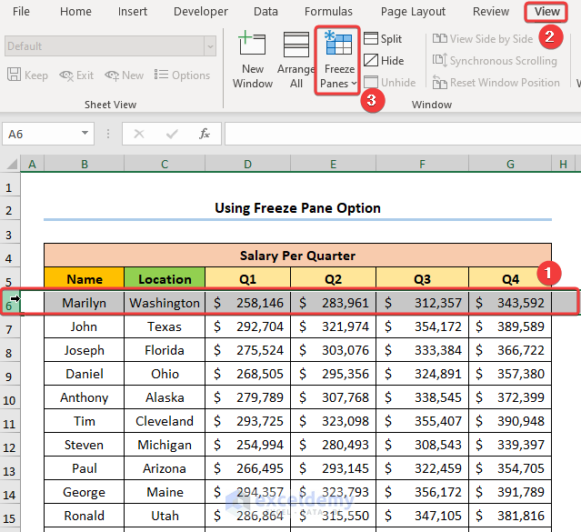
- Following this, choose the Freeze Panes option from the list.
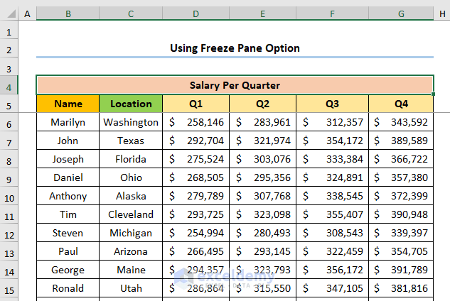
This inserts a grey line in between Rows 5 and 6. This means the top 5 Rows will stay in place even if we scroll down.
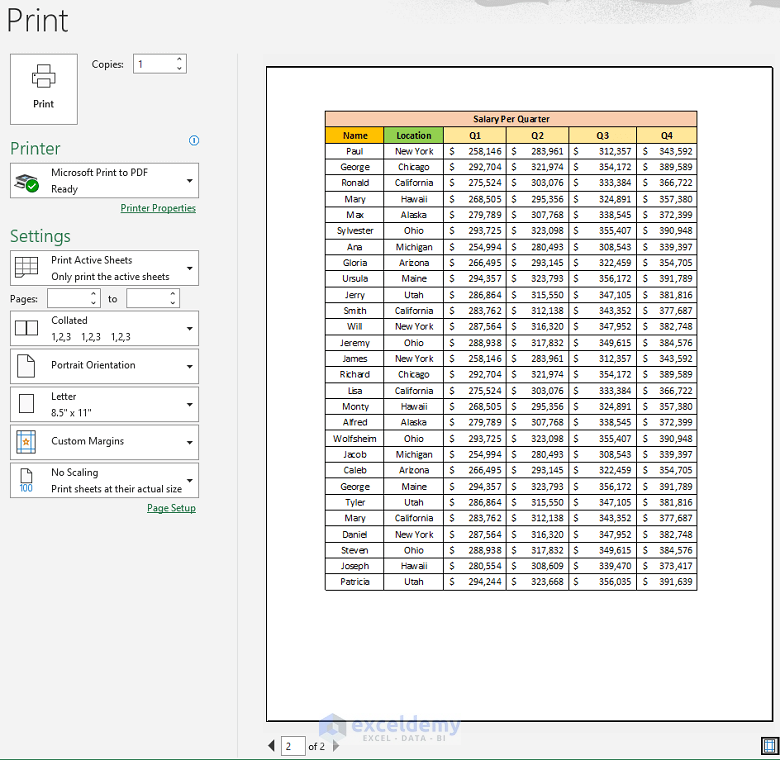
- Thirdly, press CTRL + P to open the Print option. Here, you can examine the preview pages before printing.
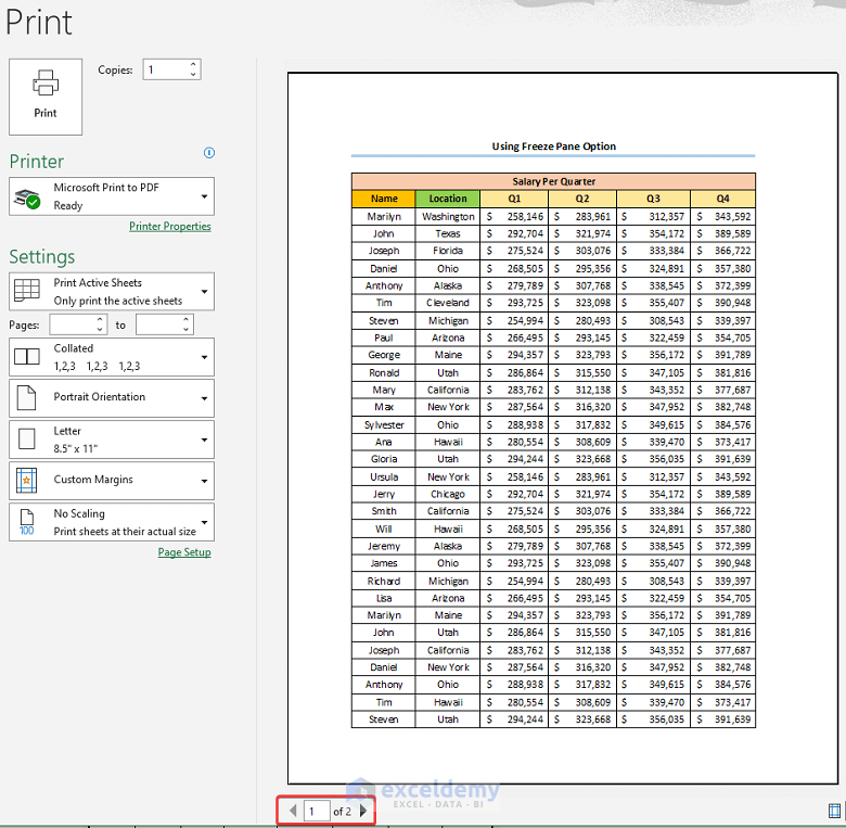
This is the second page of the worksheet.

Set Multiple Rows as Print Titles in Google Sheets
So far we’ve discussed how to set multiple rows as Print Titles in Excel. However, you can also set Print Titles using Google Sheets. It’s simple & easy, just follow along.
Steps:
- Firstly, select the cell before which you want to freeze. In this case, we chose the B5 cell.
- Secondly, go to the View tab.
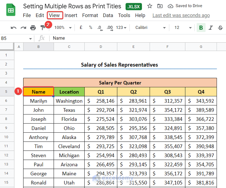
- Next, from the Freeze drop-down select the option Up to row 5.

Immediately a grey line appears which indicates the top 5 Rows are now frozen.

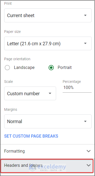
- Thirdly, press the CTRL + P shortcut on your keyboard to open the Print option.
- Now, click the Headers and footers dropdown.
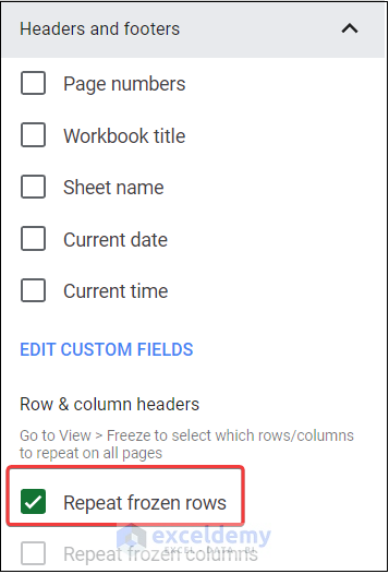
- Following this, insert a check on the Repeat frozen rows box.
- Finally, check the preview using the scroll wheel.
The image below represents the second page of the preview.
Read More: How to Set Print Titles to Repeat in Excel
Practice Section
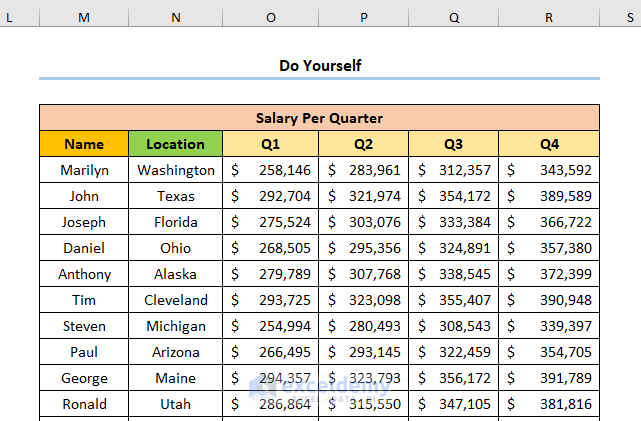
For doing practice by yourself we have provided a Practice section like below in each sheet on the right side. Please do it by yourself.
Download Practice Workbook
You can download the practice workbook from the link below.
Conclusion
This article provides quick and easy answers to how to set multiple rows as Print Titles in Excel. Make sure to download the practice files. Hope you found it helpful. Please inform us in the comment section about your experience.
Related Articles
- How to Set Print Titles in Excel
- How to Select Column A as Titles to Repeat on Each Page
- How to Print Titles in Excel Except for Last Page
- How to Remove Print Titles in Excel
<< Go Back to Print Titles | Page Setup | Print in Excel | Learn Excel
Get FREE Advanced Excel Exercises with Solutions!
