How to Select Random Sample in Excel (4 Methods)

There are several ways to Select Random Sample in Excel. Among them, we will show you 4 simple, easy, and effective methods to select random samples in Excel.

4 Methods to Select Random Sample in Excel

The following table shows Name and Salary columns. We will use 4 methods to select random name and salary from this table. Here, we used Excel 365. You can use any available Excel version.

Method-1: Using Data Analysis Toolbar to Select Random Sample

In this method, we can select random values from numeric values only using the Data Analysis toolbar. Here, we will select 5 random salaries in the Random 5 Salary column.

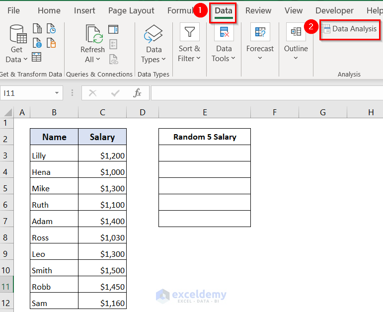
➤To begin with, we will go to the Data tab in the ribbon, and we will select Data Analysis tool.

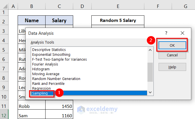
A Data Analysis window will appear.

➤ We will select Sampling as Analysis Tools.

➤ Click on OK.

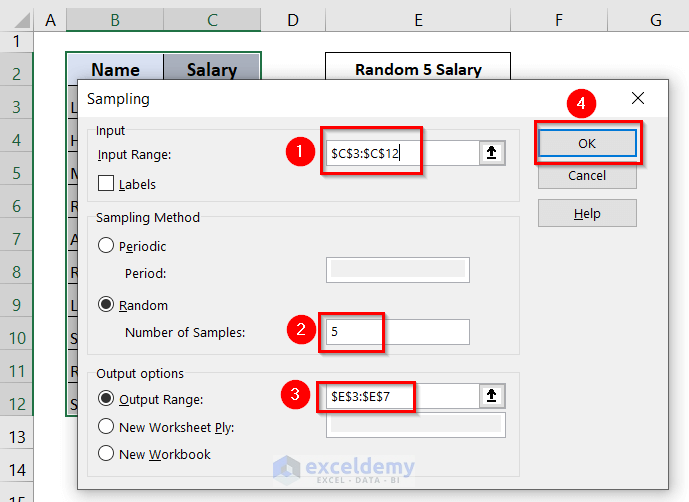
Now, a Sampling window will appear.

➤ We will select the Input Range from C3 to C12, in the Number of Sample box, we will type 5

➤ In the Output Range we will select cells from E3 to E7, and we will click OK.

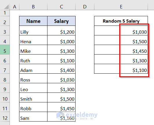
Finally, we can see 5 random salaries in the Random 5 Salary column.

Method-2: Using RAND Function

In this case, we will use the RAND function to select the top 5 random rows.

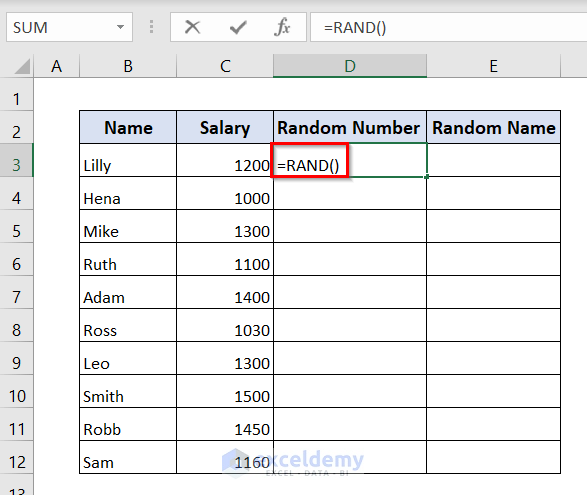
➤ First of all, we will type the following formula in cell D3.

Here, the RAND function returns in cell D3 with a random number.

➤ After that, we will press ENTER.

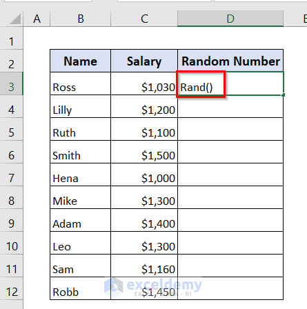
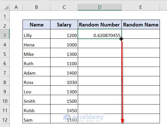
We can see a random number in cell D3.

➤ We will now drag down the formula with the Fill Handle tool.

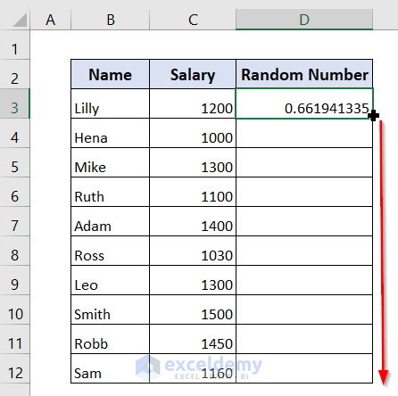
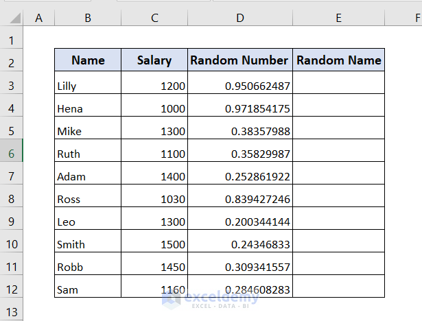
Now, we can see random numbers in the Random Number column.

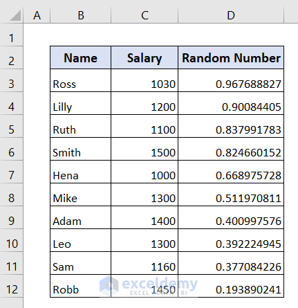
Now, we want only values in the Random Number column.

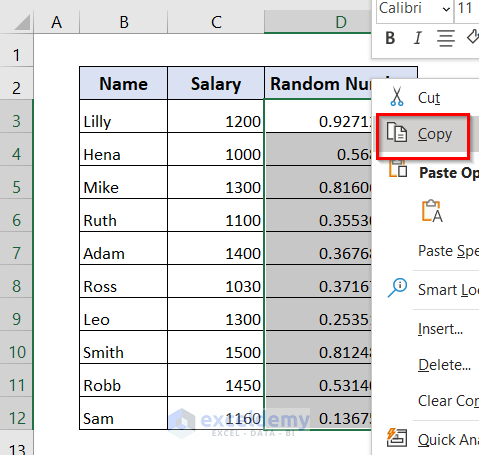
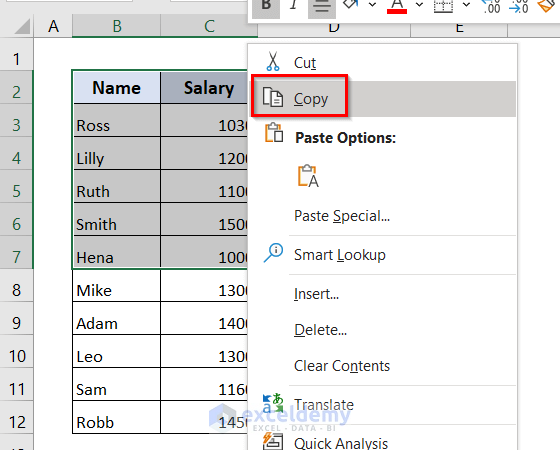
➤ To do so, we will select from cell D3 to D12, and we right click on the mouse.

➤ After that, we click on Copy.

Now, we will paste the copied number into the same cells.

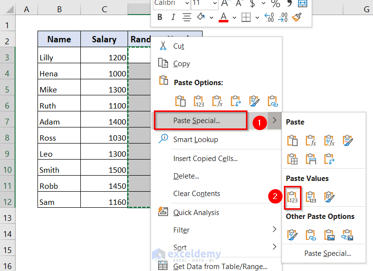
➤ We will select from cell D3 to D12, and we will right-click on the mouse.

➤ After that, we will click on Paste Special and then click on Paste Values.

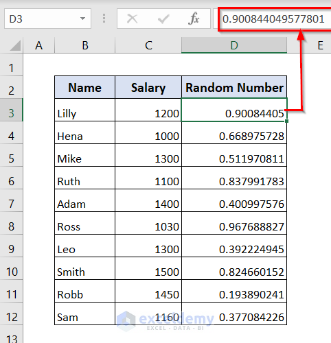
Now, we can see in the Random Number column that there is no formula in the formula bar.

Therefore, there are only values in the Random Number column.

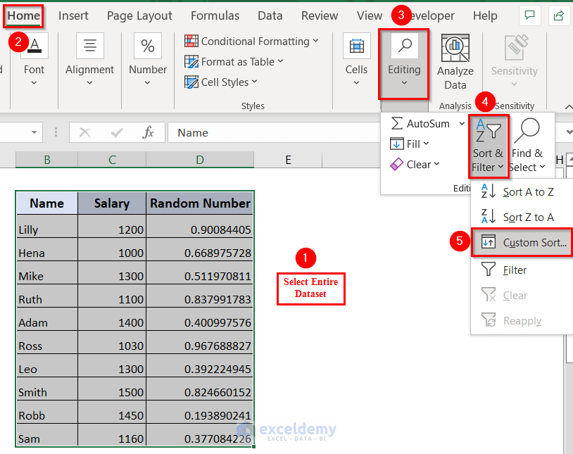
➤ Now, we will select our entire dataset, and we will go to the Home tab.

➤ After that, we will select Editing>Sort & Filter>Custom Sort.

Now, a Sort window will appear.

➤ We will select Sort by as Random Number, and Order as Largest to Smallest.

➤ Then click OK.

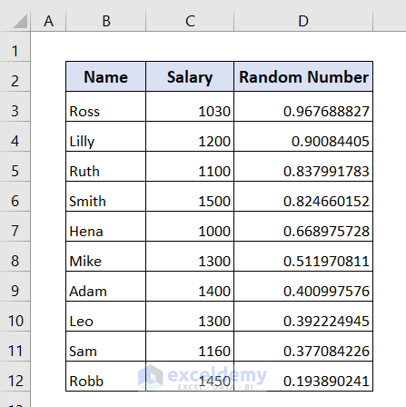
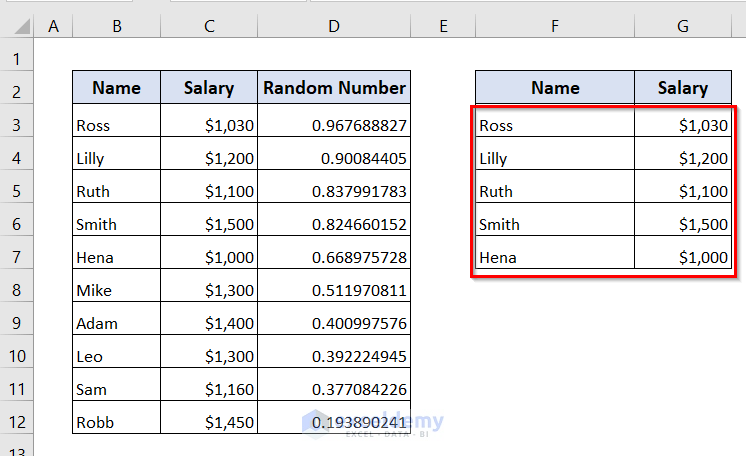
Finally, we can see the sorted Name and Salary according to the largest to smallest Random Number.

➤ Now, we will select the top 5 Name and Salary, and we will right click on the mouse, and we will select Copy.

➤ Now, we paste the top 5 Name and Salary in columns F and G.

Method-3: Using INDEX, RANDBETWEEN and ROWS Functions

In this method, we want to select a single random name.

We will use the  INDEX, RANDBETWEEN, and ROWS functions.

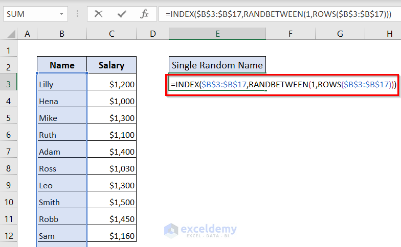
➤ First of all, we will type the following function in cell E3.

Here,

• ROWS($B$3:$B$17)→ Returns number of rows between cells B3 to B17.
• RANDBETWEEN(1,ROWS($B$3:$B$17))→ Returns a random number between 1 and number of rows.
• INDEX($B$3:$B$12, RANK(D3,$D$3:$D$12), 1)→ The number returned by RANDBETWEEN is fed to the row_num argument of the INDEX function, so it picks the value from that row. In the column_num argument, we supply 1 because we want to extract a value from the first column.

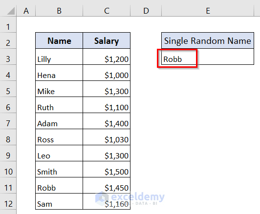
➤ Now, press ENTER.

We can see a random name Robb in our Single Random Name column.

Read More: Random Selection Based on Criteria in Excel

Method-4: Select Random Sample without Duplicates

In this method, we can select random samples without duplicates. In the following table, we want Random Number and Random Name. Here, we will use the RAND, INDEX, and RANK functions.

➤ First of all, we will type the following formula in cell D3.

➤ Press ENTER.

We can see a random number in cell D3.

➤ We can copy the formula with the Fill Handle tool.

Now, we can see random numbers in the Random Number column.

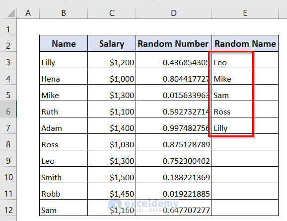
➤ Now, we will type the following formula in cell E3.

Here,

• RAND()→Returns column D with random numbers.
• RANK(D3,$D$3:$D$12)→ Returns the rank of a random number in the same row. For example, RANK(D3,$D$3:$D$12) in cell E3 gets the rank of the number in D3. When copied to D4, the relative reference D3 changes to D4 and returns the rank of the number in D4, and so on.
• INDEX($B$3:$B$12, RANK(D3,$D$3:$D$12), 1)→The number returned by RANK is fed to the row_num argument of the INDEX function, so it picks the value from that row. In the column_num argument, we supply 1 because we want to extract a value from the first column.

➤ Press ENTER.

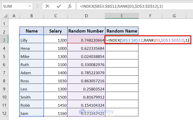
Now, we can see a random name Ruth in cell E3.

➤ We can drag down the formula with the Fill Handle tool.

Finally, we can see 5 random names in the Random Name column without duplicates.

Read More: Random Selection from List with No Duplicates in Excel

Download Workbook

Conclusion

Here, we tried to show you some easy and effective methods that will help you to select random sample in Excel. We hope you will find this article helpful. If you have any queries or suggestions, please feel free to know us in the comment section.

Random Selection in Excel: Knowledge Hub

<< Go Back to Randomize in Excel | Learn Excel