

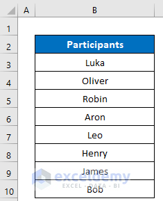
Our sample dataset represents participants in a lottery. We’ll randomly select a winner.
Method 1 – Using the INDEX and RANDBETWEEN Functions to Select from a List Randomly
Case 1.1 – Inserting the List Range Manually
Steps:
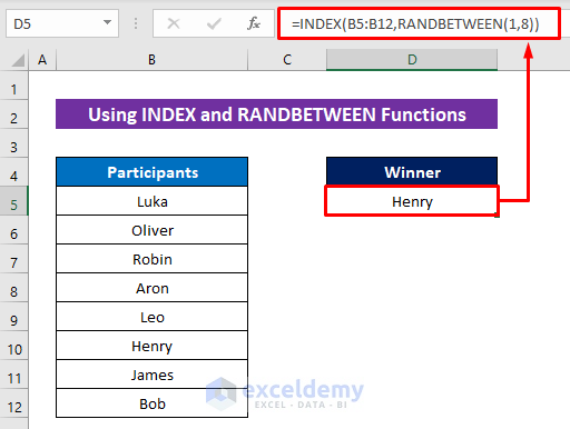
- In Cell D5, insert the following formula:
=INDEX(B5:B12,RANDBETWEEN(1,8))- Hit Enter, and you will get a random value like the image below.
Formula Breakdown:
- RANDBETWEEN(1,8)
It will return a random number among the numbers from 1 to 8.
- INDEX(B5:B12,RANDBETWEEN(1,8))
The INDEX function returns the corresponding value from the list according to the number.
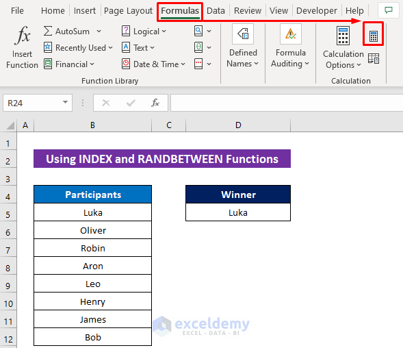
- Whenever we press Calculate Now from the Formulas tab, it will return a new random value.
Case 1.2 – Inserting the List Range Using the ROWS Function
Steps:
- Use the following formula in Cell D5:
=INDEX(B5:B12,RANDBETWEEN(1,ROWS(B5:B12)))- Hit Enter.
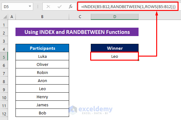
- ROWS(B5:B12)
It will return the total number of rows that used the list and actually that expresses the maximum number of the list.
- RANDBETWEEN(1,ROWS(B5:B12))
The RANDBETWEEN function will return a random number within the range.
- INDEX(B5:B12,RANDBETWEEN(1,ROWS(B5:B12)))
The INDEX function will extract the value according to the number.
Case 1.3 – Inserting the List Range Using the COUNTA Function
Steps:
- In Cell D5, insert the following formula:
=INDEX(B5:B12,RANDBETWEEN(1,COUNTA(B5:B12)))- Hit Enter.
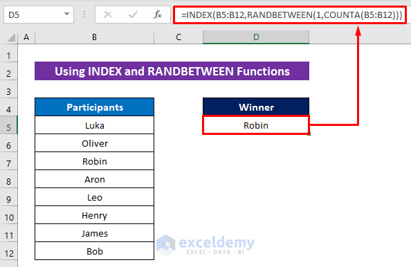
Formula Breakdown:
- This formula works as the previous formula, just using the COUNTA function instead of the ROWS function to return the highest range as the number of rows and cells in a column within the rows is the same eventually.
Method 2 – Using Excel CHOOSE and RANDBETWEEN Functions to Select from a List Randomly
Steps:
- Insert the following formula in Cell D5:
=CHOOSE(RANDBETWEEN(1,8),$B$5,$B$6,$B$7,$B$8,$B$9,$B$10,$B$11,$B$12)- Hit the Enter button.
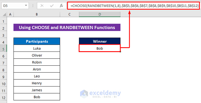
Formula Breakdown:
- RANDBETWEEN(1,8)
This will return a random number from 1 to 8.
- CHOOSE(RANDBETWEEN(1,8),$B$5,$B$6,$B$7,$B$8,$B$9,$B$10,$B$11,$B$12)
The CHOOSE function will return the value from the range of the list according to the random number.
Method 3 – Combining INDEX, RAND, and RANK Functions to Randomly Select Multiple Values
Steps:
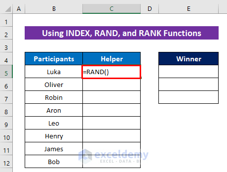
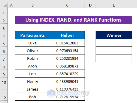
- Insert a helper column next to the list column.
- Insert the following formula to generate some random values in the new column:
=RAND()- Press the Enter button.
- Drag down the Fill Handle icon to copy the formula for the other cells.
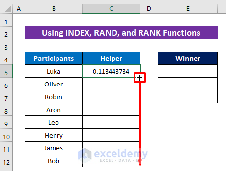
- We get random values for each name.
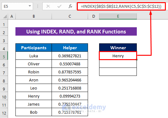
- Use the following formula in Cell E5:
=INDEX($B$5:$B$12,RANK(C5,$C$5:$C$12))- Hit Enter.
Formula Breakdown:
- RANK(C5,$C$5:$C$12)
The RANK function will create random rank numbers for every value of the range C5:C12.
- INDEX($B$5:$B$12,RANK(C5,$C$5:$C$12))
The INDEX function will extract the value according to the number.
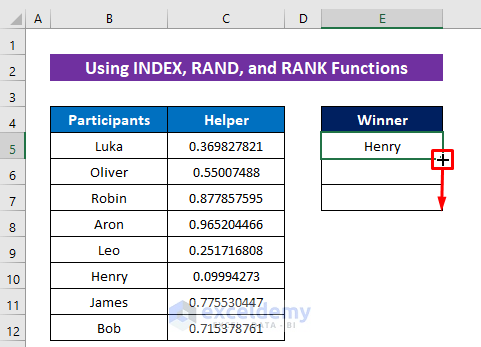
- Use the Fill Handle tool to copy the formula and get the other two random values.
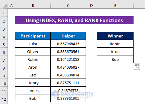
- We got three random values.
Method 4 – Randomly Select Multiple Unique Values Using INDEX, RAND, RANK, and MATCH Functions
Steps:
- Use Method 3 to fill column C.
- Insert a new helper columns.
- Use the following formula in Cell D5:
=RANK(C5,$C$5:$C$12)- Hit Enter.
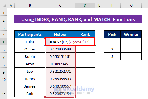
- Use the Fill Handle tool to copy the formula.
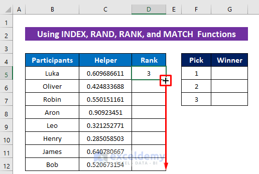
- This gives each person a random rank.
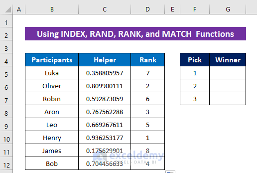
- Insert the following formula in Cell G5:
=INDEX($B$5:$D$12,MATCH(F5,$D$5:$D$12,0),1)- Hit the Enter button to get the first random value.
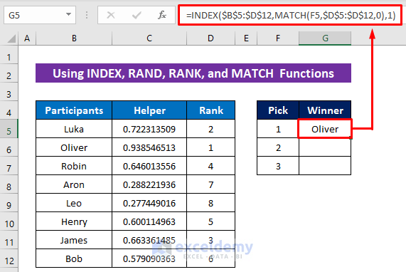
Formula Breakdown:
- MATCH(F5,$D$5:$D$12,0)
The MATCH function will return the relative position from the array according to the specific value.
- INDEX($B$5:$D$12,MATCH(F5,$D$5:$D$12,0),1)
The INDEX function will extract the corresponding value according to the relative position.
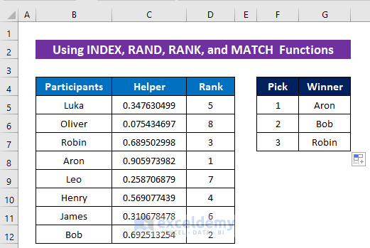
- Use the Fill Handle tool to get the other two random values.
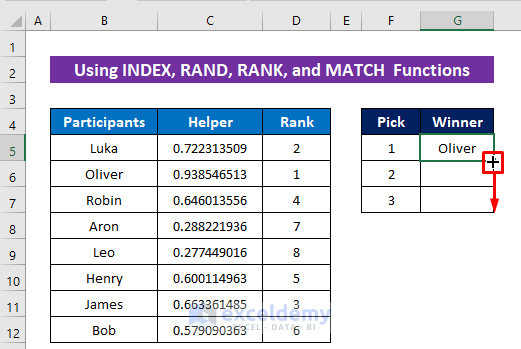
- We got three different random names. Each time you will recalculate, you will get new names.
Method 5 – Using XLOOKUP to Randomly Select Multiple Values Without Duplicates in Excel
Steps:
- Use Method 3 and 4 to fill in two helper columns C and D.
- Use the formula given below in Cell G5:
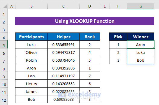
=XLOOKUP(F5:F7,D5:D12,B5:B12)- Press the Enter button to get the array.
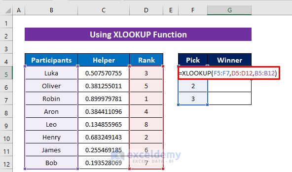
- Here are our random names as an array output.
Download the Practice Workbook
<< Go Back to Random Selection in Excel | Randomize in Excel | Learn Excel
Get FREE Advanced Excel Exercises with Solutions!


Lots of great info, presented clearly. Thanks.
I was surprised that there was no evaluation of which methods work best. For example, if your list of items changes, how easy is it to change the formula.
Or the fact that “CHOOSE(RANDBETWEEN(1,8),$B$5,$B$6,$B$7,$B$8,$B$9,$B$10,$B$11,$B$12)” is truly awful and no one should ever use it. It belongs in Reddit /r/techicallytrue
Hello Bob Dragon,
Thank you for the thoughtful feedback. You make a valid point—the article should explain not only how each method works, but also how practical and maintainable it is when the source list changes.
The CHOOSE and RANDBETWEEN method is included mainly to demonstrate another possible approach. However, we agree that manually listing every cell makes it unsuitable for a growing or frequently changing list. In most cases, the INDEX formula using ROWS is a much better option:
=INDEX(B5:B12,RANDBETWEEN(1,ROWS(B5:B12)))
For even greater flexibility, the source data can be converted into an Excel Table so that the formula automatically adjusts when items are added or removed. We appreciate your suggestion and will consider adding a comparison of the methods and their limitations to make the article more useful.
Regards,
ExcelDemy