Method 1 – Random Selection Based on Criteria Using INDEX Function
Steps:
- Type the following formula in cell G8.
=INDEX(B5:B15,LARGE(IF(E5:E15=G5,ROW(E5:E15)ROW(E5)+1),INT(RAND()*COUNTIF(E5:E15,G5)+1)))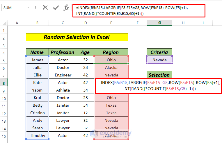
- Press the ENTER key. If you are using Excel version 2019 or Lower the press CTRL+SHIFT+ENTER as this is an array formula. You will not find any curly braces in an upgraded version of Excel like Excel 2016, Microsoft 365, etc.
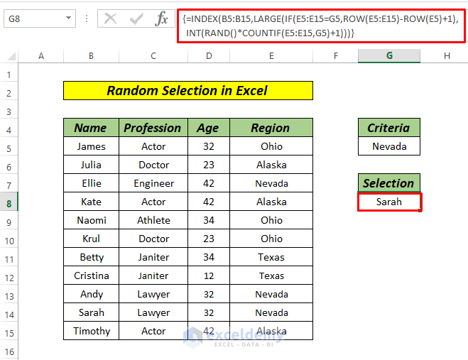
- IF(E5:E15=G5,ROW(E5:E15)-ROW(E5)+1) formula gives us the output as.{FALSE;FALSE;3;FALSE;FALSE;FALSE;FALSE;FALSE;9;10;FALSE}.
- The formula INT(RAND()*COUNTIF(E5:E15,G5)+1) gives us the output as 10. Here, INT(RAND() function automatically generates a random integer number.
- =INDEX(B5:B15,10) will generate a random name Sarah, which will change every time we refresh or press ENTER in the formula bar.
Case 2: INDIRECT-RANDBETWEEN Combination for Random Selection
Steps:
- Type the following formula in cell G9.
=INDEX(B5:B15,LARGE(IF(E5:E15=G5,ROW(E5:E15)ROW(E5)+1),INT(RAND()*COUNTIF(E5:E15,G5)+1)))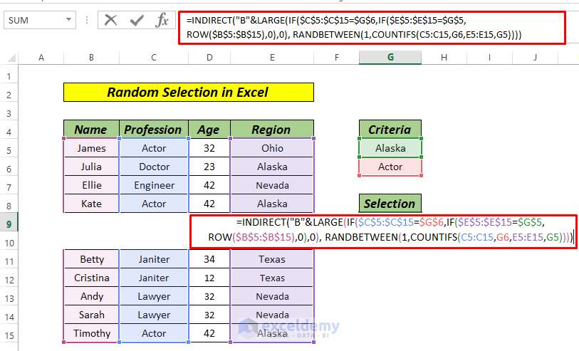
- Press the ENTER key or CTRL+SHIFT+ENTER for Excel versions lower than 2019.
- “B” in the formula indicates the Name column.
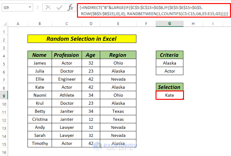
- Formula RANDBETWEEN(1,COUNTIFS(C5:C15,G6,E5:E15,G5)) returns us a random value 2.{0;0;0;8;0;0;0;0;0;0;15} is the value we get from the formula IF($C$5:$C$15=$G$6,IF($E$5:$E$15=$G$5,ROW($B$5:$B$15),0),0).
- =INDIRECT(“B”&15) gives us the final result as Kate.
Method 3 – AGGREGATE Function for Random Selection Based on Criteria
Steps:
- Type the following formula in cell G10.
=INDEX(B4:B15,AGGREGATE(15,3,(E5:E15<>"Nevada")*ROW(E5:E15), RANDBETWEEN(COUNTIF(E5:E15,"Nevada")+1,COUNTA(E5:E15))))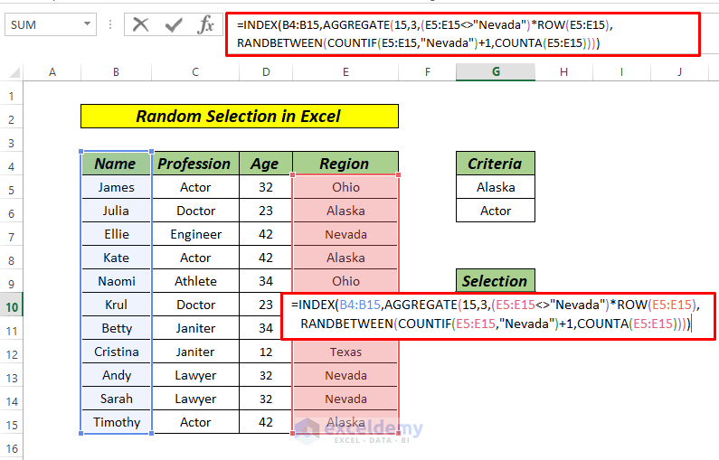
- Press the ENTER key. If you are using Excel version 2019 or Lower the press CTRL+SHIFT+ENTER as this is an array formula.
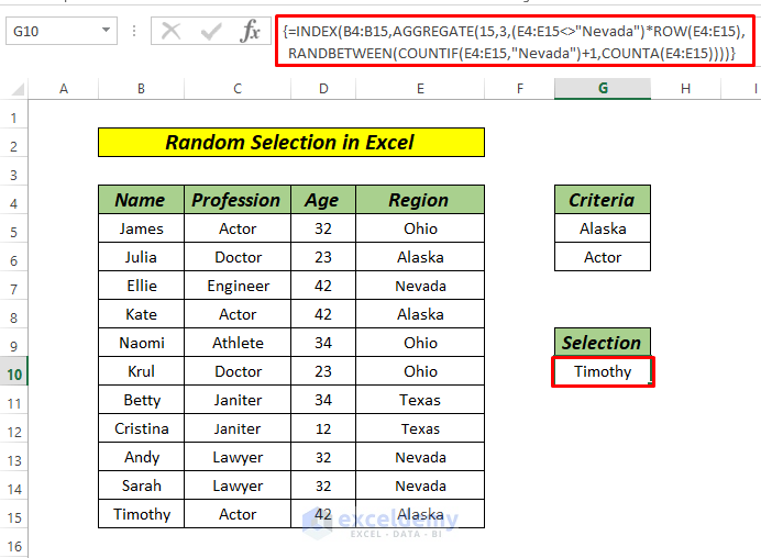
- RANDBETWEEN(COUNTIF(E5:E15,”Nevada”)+1,COUNTA(E5:E15)) formula gives us an output 5 and AGGREGATE(15,3,(E5:E15<>”Nevada”)*ROW(E5:E15),RANDBETWEEN(COUNTIF(E5:E15,”Nevada”)+1,COUNTA(E5:E15))) yield the output as 11, which is clearly the row number of Timothy (Count from the Header column).
- =INDEX(B4:B15,11) will give the result as Timothy.
Download Practice Workbook
<< Go Back to Random Selection in Excel | Randomize in Excel | Learn Excel
Get FREE Advanced Excel Exercises with Solutions!
