Method 1 – Using RAND, INDEX, and RANK.EQ Functions for Random Selection without Duplicates
Steps:
➤ For generating random unique numbers type the following function in cell C4.
=RAND()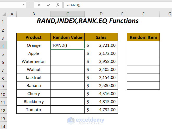
➤ Press ENTER and drag down the Fill Handle tool.
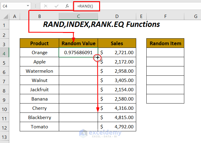
Get the following random numbers and notice the effect of the volatile function RAND in changing the numbers after each calculation. You can see that before applying the AutoFill feature the value in the cell was 0.975686091 and after applying the value changed to 0.082805271.
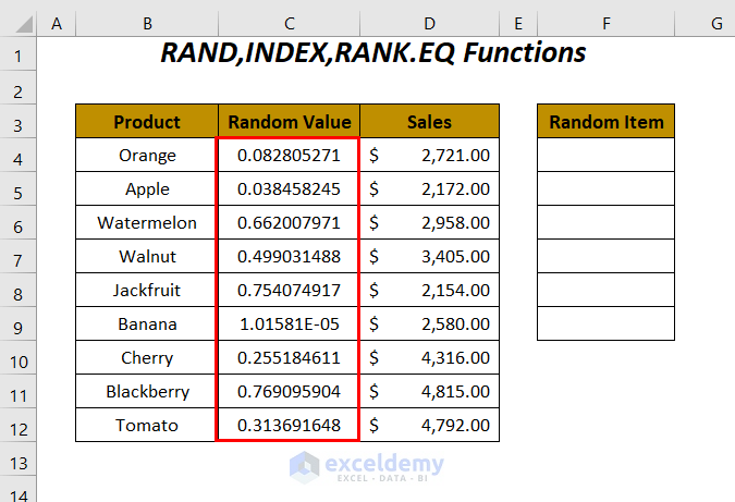
This function will automatically change those random values and will affect our selection. To prevent this, you can paste them as values.
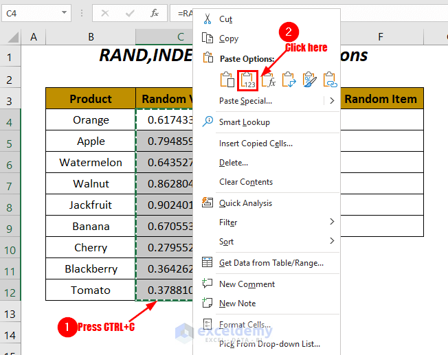
➤ Select the range of the random values and press CTRL+C.
➤ Right-click on your mouse and select the Values option from different Paste Options.
Get the fixed random values, and now, using them, we will make our random selection.
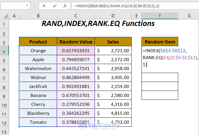
➤ Type the following formula in cell F4.
=INDEX($B$4:$B$12,RANK.EQ(C4,$C$4:$C$12),1)$B$4:$B$12 is the range of products, and $C$4:$C$12 is the range of random values.
RANK.EQ(C4,$C$4:$C$12)becomes
RANK.EQ(0.617433431,$C$4:$C$12)→RANK.EQreturns the rank of the value0.617433431among other values in the range$C$4:$C$12.
Output →6
INDEX($B$4:$B$12,RANK.EQ(C4,$C$4:$C$12),1)becomes
INDEX($B$4:$B$12,6,1)→INDEXreturns the value of cellB9at the intersection ofRow 6andColumn 1in the range$B$4:$B$12.
Output →Banana
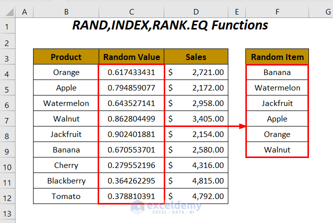
➤ Press ENTER and drag down the Fill Handle tool.
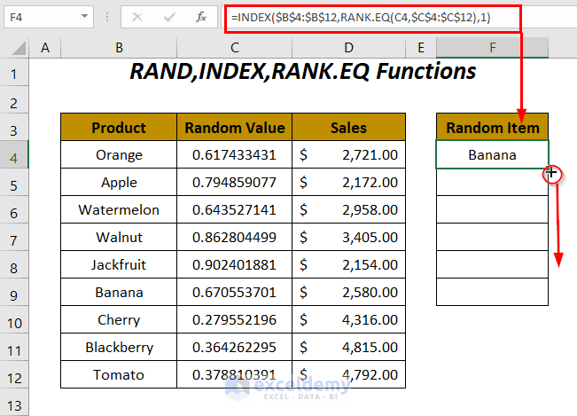
We made our random selection of 6 products among the 9 products avoiding any duplicate selection.
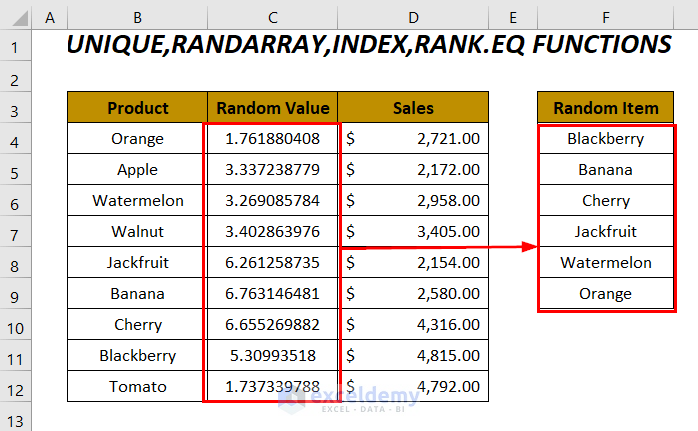
Method 2 – Using UNIQUE, RANDARRAY, INDEX, and RANK.EQ Functions
Steps:
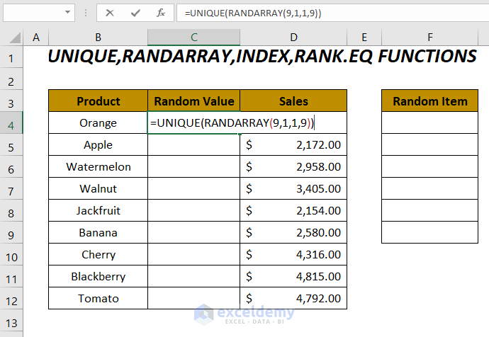
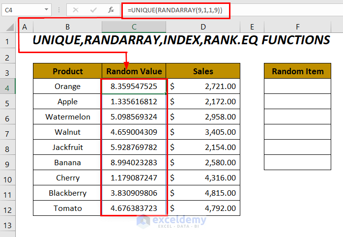
➤ To have the random unique numbers type the following function in cell C4.
=UNIQUE(RANDARRAY(9,1,1,9))9 is the total number of rows, 1 is the number of columns, 1 is the minimum number, and 9 is the maximum number. Then RANDARRAY will give an array of this size of random numbers and UNIQUE will return the unique numbers from this array.
➤ After pressing ENTER and dragging down the Fill Handle tool you will have the following random numbers in the Random Value column.
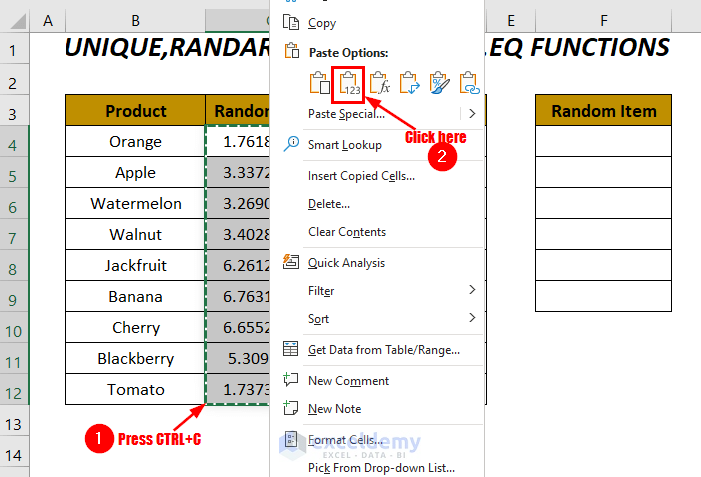
As RANDARRAY is a volatile function, it will automatically change those random values and will also affect our selection. To prevent this, we will paste them as values.
➤ Select the range of the random values and press CTRL+C.
➤Right-click on your mouse and select the Values option from different Paste Options.
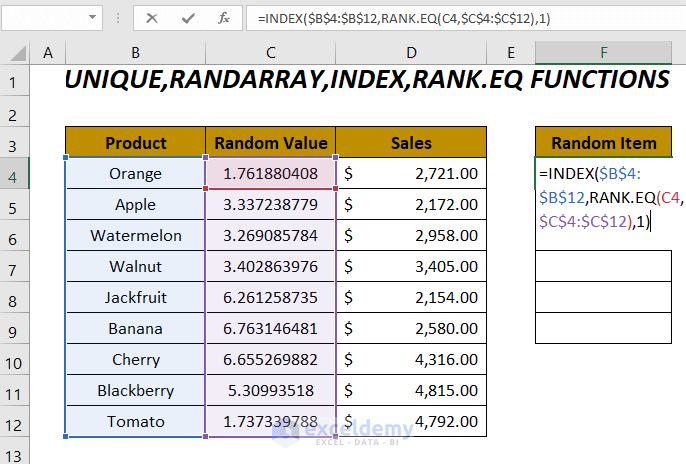
Get the fixed random values, and now, using them, we will make our random selection.
➤ Type the following formula in cell F4.
=INDEX($B$4:$B$12,RANK.EQ(C4,$C$4:$C$12),1)$B$4:$B$12 is the range of products, and $C$4:$C$12 is the range of random values.
RANK.EQ(C4,$C$4:$C$12)becomes
RANK.EQ(1.761880408,$C$4:$C$12)→RANK.EQreturns the rank of the value1.761880408among other values in the range$C$4:$C$12.
Output →8
INDEX($B$4:$B$12,RANK.EQ(C4,$C$4:$C$12),1)becomes
INDEX($B$4:$B$12,8,1)→INDEXreturns the value of cellB11at the intersection ofRow 8andColumn 1in the range$B$4:$B$12.
Output →Blackberry
➤ Press ENTER and drag down the Fill Handle tool.
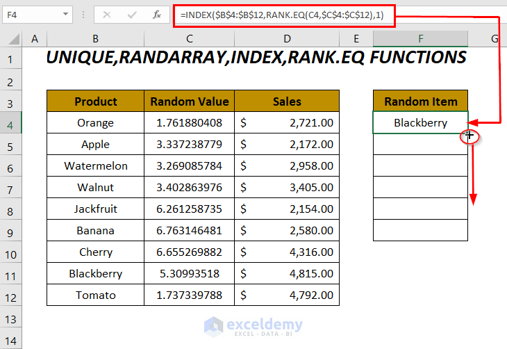
We did our random selection of the products without duplicates in the Random Item column.
The UNIQUE function and the RANDARRAY function are available only for Microsoft Excel 365 and Excel 2021 versions.
Method 3 – Random Selection with No Duplicates Using RAND, INDEX, RANK.EQ, and COUNTIF
Steps:
➤ For generating random unique numbers apply the following function in the cells of the Random Value column.
=RAND()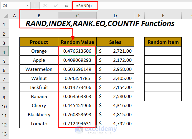
As RAND is a volatile function, it will automatically change those random values and will also affect our selection. To prevent this, we will paste them as values.
➤ Select the range of the random values and press CTRL+C.
➤ Right-click on your mouse and select the Values option from different Paste Options.
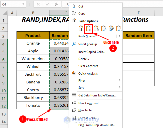
You will have stable random values, which you can use to make our random selection.
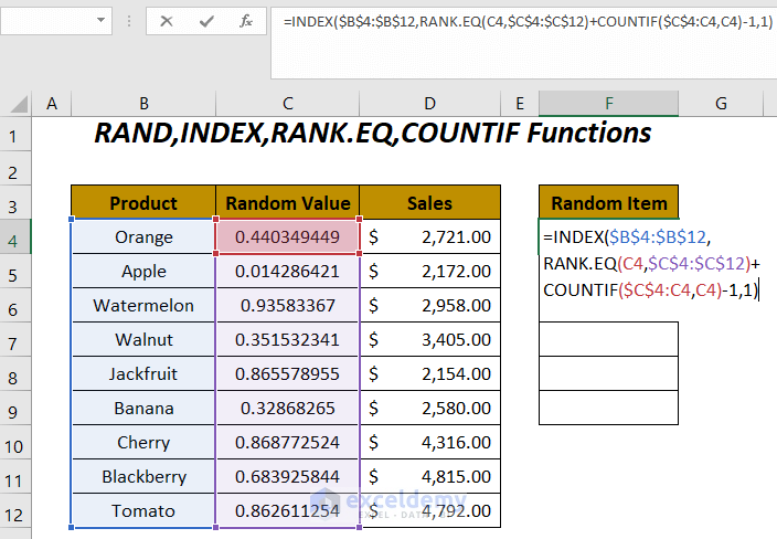
➤ Apply the following formula in cell F4.
=INDEX($B$4:$B$12,RANK.EQ(C4,$C$4:$C$12)+COUNTIF($C$4:C4,C4)-1,1)$B$4:$B$12 is the range of products, and $C$4:$C$12 is the range of random values.
RANK.EQ(C4,$C$4:$C$12)becomes
RANK.EQ(0.440349449,$C$4:$C$12)→RANK.EQreturns the rank of the value0.440349449among other values in the range$C$4:$C$12.
Output →6COUNTIF($C$4:C4,C4) becomes
COUNTIF($C$4:C4,0.440349449)→counts the number of cells having the value440349449in the range$C$4:C4
Output →1RANK.EQ(C4,$C$4:$C$12)+COUNTIF($C$4:C4,C4)-1becomes
6+1-1 → 6INDEX($B$4:$B$12,RANK.EQ(C4,$C$4:$C$12)+COUNTIF($C$4:C4,C4)-1,1)becomes
INDEX($B$4:$B$12,6,1)→INDEXreturns the value of cellB9at the intersection ofRow 6andColumn 1in the range$B$4:$B$12.
Output →Banana
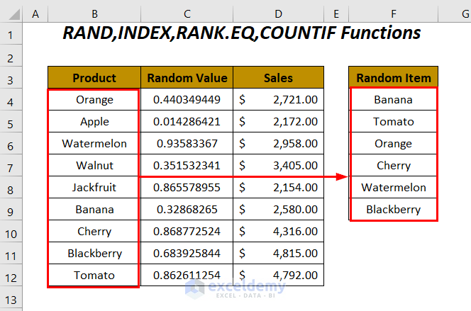
➤ Press ENTER and drag down the Fill Handle tool.
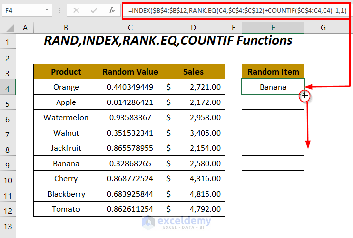
Our random selection of 6 products among the 9 products avoiding any duplicate selection.
Method 4 – Using Combination of INDEX, SORTBY, RANDARRAY, ROWS, and SEQUENCE Functions
Steps:
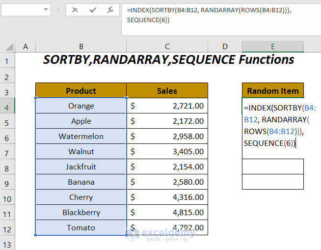
➤ Use the following formula in cell E4.
=INDEX(SORTBY(B4:B12, RANDARRAY(ROWS(B4:B12))), SEQUENCE(6))$B$4:$B$12 is the range of products.
ROWS(B4:B12)→ returns the total row numbers in this range
Output → 9
RANDARRAY(ROWS(B4:B12))becomes
RANDARRAY(9)→ generates random 9 numbers
Output →{0.94536; 0.51383; 0.86142; 0.78644; 0.34980; 0.48125; 0.63824; 0.24971; 0.045946}
SORTBY(B4:B12, RANDARRAY(ROWS(B4:B12)))becomes
SORTBY({“Orange”, “Apple”, “Watermelon”, “Walnut”, “Jackfruit”, “Banana”, “Cherry”, “Blackberry”, “Tomato”}, {0.94536; 0.51383; 0.86142; 0.78644; 0.34980; 0.48125; 0.63824; 0.24971; 0.045946})
Output →{“Watermelon”, “Blackberry”, “Walnut”, “Apple”, “Jackfruit”, “Banana”, “Cherry”, “Walnut”, “Tomato”, “Orange”}
SEQUENCE(6)→ gives a range of serial numbers from 1 to 6
Output →{1; 2; 3; 4; 5; 6}
INDEX(SORTBY(B4:B12, RANDARRAY(ROWS(B4:B12))), SEQUENCE(6))becomes
INDEX(SORTBY({“Watermelon”, “Blackberry”, “Walnut”, “Apple”, “Jackfruit”, “Banana”, “Cherry”, “Walnut”, “Tomato”, “Orange”}, {1; 2; 3; 4; 5; 6})
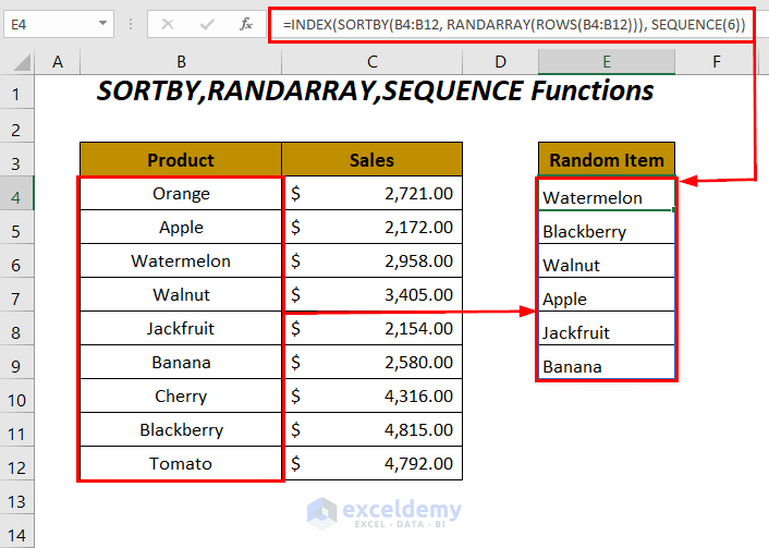
Output →{“Watermelon”, “Blackberry”, “Walnut”, “Apple”, “Jackfruit”, “Banana”}
After pressing ENTER, you will get 6 random products in the Random Item column.
The SORTBY function and the RANDARRAY function are available only for Microsoft Excel 365 and Excel 2021 versions.
Method 5 – Selection of a Whole Row from a List without Duplicates
Steps:
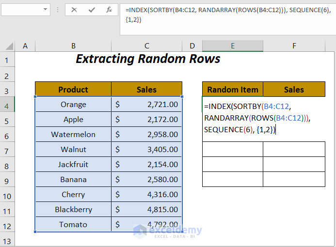
➤ Write down the following formula in cell E4.
=INDEX(SORTBY(B4:C12, RANDARRAY(ROWS(B4:C12))), SEQUENCE(6), {1,2})B4:C12 is the range of products and sales values.
ROWS(B4:C12)→ returns the total row numbers in this range
Output → 9
RANDARRAY(ROWS(B4:B12))becomes
RANDARRAY(9)→ generates random 9 numbers
Output →{0.69680; 0.04111; 0.23072; 0.54573; 0.18970; 0.98737; 0.29843; 0.59124; 0.60439}
SORTBY(B4:B12, RANDARRAY(ROWS(B4:B12)))becomes
SORTBY({“Orange”, 2721; “Apple”, 2172; “Watermelon”, 2958;“Walnut”, 3405; “Jackfruit”, 2154; “Banana”, 2580; “Cherry”, 4316; “Blackberry”, 4815; “Tomato”, 4792}, {0.94536; 0.51383; 0.86142; 0.78644; 0.34980; 0.48125; 0.63824; 0.24971; 0.045946})
Output →{“Tomato”, 4792; “Walnut”, 3405; “Blackberry”, 4815; “Banana”, 2580; “Apple”, 2172; “Cherry”, 4316; “Orange”, 2721; “Jackfruit”, 2154; “Watermelon”, 2958}
SEQUENCE(6)→ gives a range of serial numbers from 1 to 6
Output →{1; 2; 3; 4; 5; 6}
INDEX(SORTBY(B4:C12, RANDARRAY(ROWS(B4:C12))), SEQUENCE(6), {1,2})becomes
INDEX(SORTBY({“Tomato”, 4792; “Walnut”, 3405; “Blackberry”, 4815; “Banana”, 2580; “Apple”, 2172; “Cherry”, 4316; “Orange”, 2721; “Jackfruit”, 2154; “Watermelon”, 2958}, {1; 2; 3; 4; 5; 6}, {1,2})
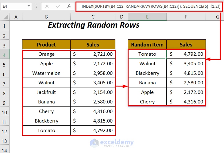
Output →{“Tomato”, 4792; “Walnut”, 3405; “Blackberry”, 4815; “Banana”, 2580; “Apple”, 2172; “Cherry”, 4316}
After pressing ENTER, you will get any random 6 products and their corresponding sales values.
Download Practice Workbook
<< Go Back to Random Selection in Excel | Randomize in Excel | Learn Excel
Get FREE Advanced Excel Exercises with Solutions!
