We often need to randomly select data from our Excel sheet, especially text data. Microsoft Excel does not offer any dedicated function to select random data. In this article, we will discuss how to randomly select participants in Excel in 4 different ways.
In this article, we will learn 4 handy ways to randomly select participants in Excel. Firstly, we will use a combination of the INDEX, RANDBETWEEN, and ROWS functions. Then, we will combine the INDEX, RANDBETWEEN, and COUNTA functions to do the task. After that, we will opt for the RANK function to select random text data. Finally, we will resort to a VBA code to select data randomly. We will use the sample data below to demonstrate the methods.

1. Using INDEX, RANDBETWEEN, and ROWS Functions to Randomly Select Participants in Excel
In this method, we will combine three functions to randomly select participants in excel. The INDEX function extracts a value from a table or range, or a reference to a value, and returns it. The RANDBETWEEN function returns an integer number at random within the range that the user specifies. Finally, the ROWS function returns the row number of a reference.
Steps:
- To begin with, select the E5 cell and write down the following formula,
=INDEX($B$5:$B$10,RANDBETWEEN(1,ROWS($B$5:$B$10)),1)- Then, hit Enter.

- Consequently, the cell will show a randomly selected participant.
- You can copy the formula down to select multiple participants.

🔎 Formula Breakdown:
- ROWS($B$5:$B$10): The Rows function returns the number of rows within a range. Here, the function returns the total number of rows in the range (B5:B10). The result is 5.
- RANDBETWEEN(1,ROWS($B$5:$B$10)): The RANDBETWEEN function returns any random number within the range that users specify as an argument. Here, the range is between 1 and 5. The 5 value is returned by the ROWS function.
- INDEX($B$5:$B$10,RANDBETWEEN(1,ROWS($B$5:$B$10)),1): The INDEX function displays the data at a particular cell. Here, the first argument of the INDEX function is a range. This means the function will go through this range to look for the cell whose data we want to display. The second argument is the row number. Here, the RANDBETWEEN function returns any integer number between 1 to 5 as the row number. That is why the data that the INDEX function will show will also be random data. Finally, the column number is 1 since we are getting the data from one column.
2. Combining Excel INDEX, RANDBETWEEN, and COUNTA Functions to Randomly Select Participants
In this instance, we will combine the COUNTA function with the previously mentioned two functions, the INDEX function, and the RANDBETWEEN function, to select participants randomly in Excel. The COUNTA function counts the number of non-empty cells within a range.
Steps:
- Firstly, select the E5 and write the following formula down,
=INDEX($B$5:$B$10,RANDBETWEEN(1,COUNTA($B$5:$B$10)),1)- After that, hit Enter.

- Consequently, you will find a randomly selected participant in the E5 cell.
- Move the cursor down to select more random participants.

🔎 Formula Breakdown:
- COUNTA($B$5:$B$10): The COUNTA function returns the number of cells that are not empty within a range. Here, the function returns the total number of non-empty cells in the range B5:B10. The result is 5.
- RANDBETWEEN(1,COUNTA($B$5:$B$10)): The RANDBETWEEN function returns any random number within the range that users specify as an argument. Here, the range is between 1 and 5. The 5 value is returned by the COUNTA function.
- INDEX($B$5:$B$10,RANDBETWEEN(1,COUNTA($B$5:$B$10)),1): The INDEX function displays the data at a particular cell. Here, the first argument of the INDEX function is a range. This means the function will go through this range to look for the cell in which data we want to display. The second argument is the row number. Here, the RANDBETWEEN function returns any integer number between 1 to 5 as the row number. That is why the data that the INDEX function will show will also be random data. Finally, the column number is 1 since we are getting the data from one column.
3. Applying the RANK Function to Randomly Select Participants Without Duplicates
If you want to have multiple randomly selected data without duplication, then this method will be useful for you. Here, we use the RAND function and the RANK function to display unique random participants. The RAND function generates random numbers. The RANK function ranks a particular number within a list of numbers or an array of numbers.
Steps:
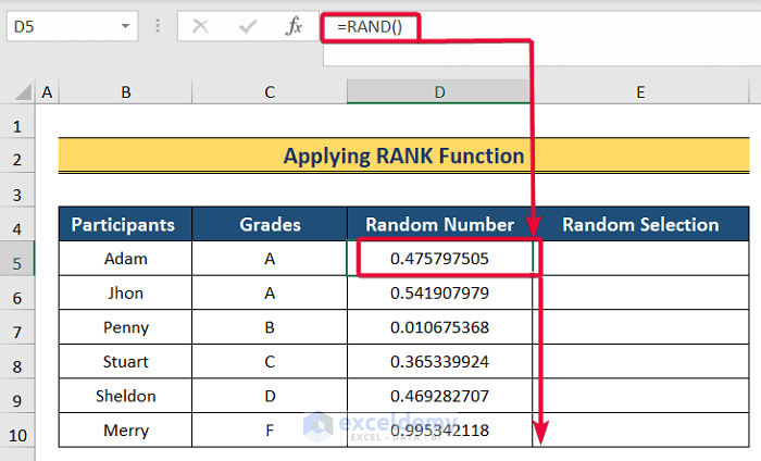
- Firstly, select the D5 cell and write down,
=RAND()- Then, hit the Enter button.

- Consequently, you will have a random number in the D5 cell.
- Next, move the cursor down to the last dataset to fill the column with random numbers.
- After that, select the E5 cell and write the following formula:
=INDEX($B$5:$B$10, RANK(D5,$D$5:$D$10), 1)- Then, press Enter.
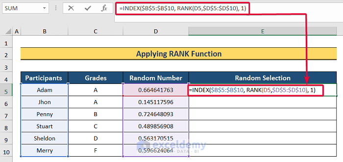
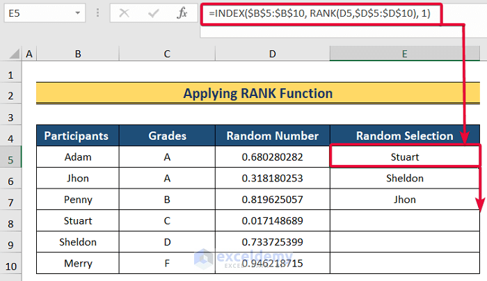
- As a result, you will get a random participant name in the cell.
- Place your cursor below the number of cells that will correspond to the participants you want to select.
🔎 Formula Breakdown:
- RANK(D5,$D$5:$D$10): The Rank function ranks the data in cell D5 among the cells in the D5:D10 Then, if we move the cursor down by one, the relative cell reference changes from D5 to D6 but the range remains as the range contains an absolute cell reference. The RANK function ranks the cells gradually, and the E5 cell gets the rank of the number in the D5 cell.
- INDEX($B$5:$B$10, RANK(D5,$D$5:$D$10), 1): The rank of the E5 cell is taken as the row_num of the INDEX function. Since the rank number is a random number, the row number will also be random. Thus the formula returns randomly selected participants.
4. Using VBA Code to Randomly Select Participants in Excel
In this method illustration, we will resort to a VBA code to solve the problem. This VBA code will allow us to randomly select a participant in Excel.
Steps:
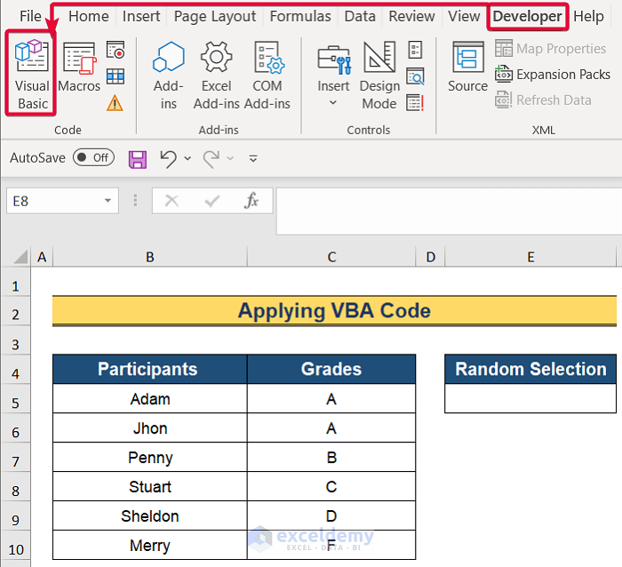
- Firstly, go to the Developer tab in the ribbon.
- From there, select the Visual Basics tab.
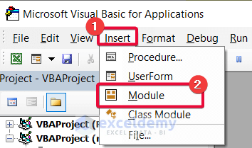
- After that, in the Visual Basic tab, click on Insert.
- Then, select the Module option.
- Consequently, a coding module will appear.
- In the coding module, write down the following code.
- Then, save the code.
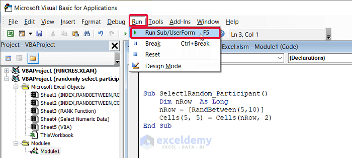
Sub Select1Random_Participant()
    Dim nRow  As Long
    nRow = [RandBetween(5,10)]
    Cells(5, 5) = Cells(nRow, 2)
End Sub
- Finally, go to the Run tab and click on it.
- From the drop-down option, select the Run command to run the code.
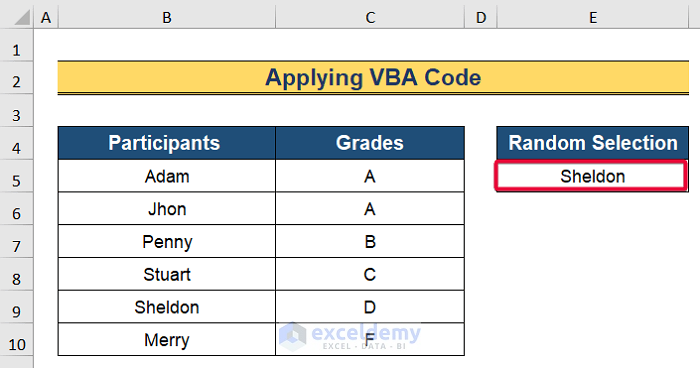
- Consequently, you will find the name of a randomly selected participant in the E5.
How to Use Data Analysis Toolbar to Randomly Select Numeric Data
In the previous methods, we selected text data. In this method, we will use the Data Analysis toolbar to select random numeric data.
Steps:
- Firstly, go to the Data tab in the ribbon.
- Then, select the Data Analysis toolbar.
- Consequently, the Data Analysis dialogue box will appear.

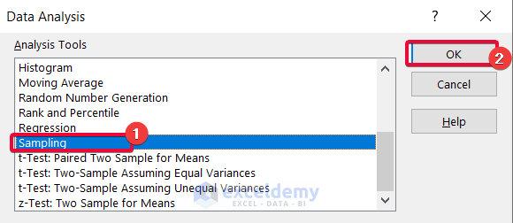
- Afterward, from the dialogue box, select Sampling.
- Finally, click OK.
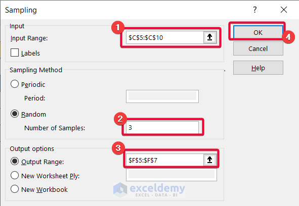
- As a result, the Sampling window will appear.
- From the window, select ($C5:$C10) as the Input Range.
- Write down 3 as the Number of samples under the Random option.
- Then, select ($F5:$F7) as the Output Range.
- Finally, click OK.
- Consequently, you will find 3 random data appearing in the selected range.

Download Practice Workbook
You can download the practice workbook from here.
Conclusion
In this article, we have talked about 4 easy ways randomly to select participants in Excel. This will allow the Excel users to randomly select text data from their dataset.
<< Go Back to Random Selection in Excel | Randomize in Excel | Learn Excel
Get FREE Advanced Excel Exercises with Solutions!
