Microsoft Excel is a powerful software. We can perform numerous operations on our datasets using excel tools and features. There are many default Excel Functions that we can use to create formulas. Many educational institutions and business companies use excel files to store valuable data. Sometimes, we need to perform a reverse what-if analysis. There are multiple ways available to carry out the operation. This article will show you all 2 handy approaches to doing Reverse What-If Analysis in Excel.
How to Do Reverse What-If Analysis in Excel: 2 Handy Approaches
Usually, the what-if analysis is done to see the changes in the results or output end when we modify or alter the input ends. But, in the case of reverse what-if analysis, the output is kept at a fixed value or target. Now, to keep the output fixed, we need to make some adjustments to the input. We can easily solve such problems in excel with the multiple useful tools it offers. Therefore, go through the article to learn about all the possible ways to do Reverse What-If Analysis in Excel.
1. Perform Reverse What-If Analysis with Goal Seek in Excel
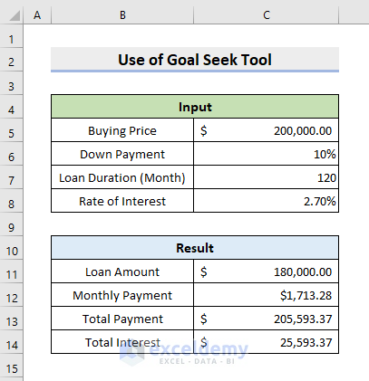
In our first approach, we’ll use the Goal Seek tool. To illustrate, we’ll use a sample dataset. For instance, the dataset contains data on a loan, its down payment, interest rate, etc. Here, $1713.28 is the monthly payment. This amount might be excessive for some people. We want to set this to $1500. Lowering the Buying Price is a way to solve the issue. So, we’ll be doing a reverse what-if analysis here as we’ll modulate the input for a fixed output. Hence, follow the steps below to perform the task.
STEPS:
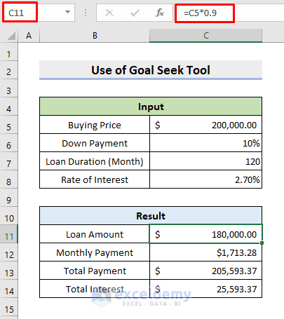
- Before we begin with the process, notice cell C11.
- The formula is:
=C5*0.9- This is the loan-to-value amount after depositing the down payment of 10%.
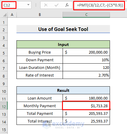
- Again, a formula is required to calculate the monthly payment in cell C12 which will link the cell to the Buying Price in cell C5.
- Otherwise, the Goal Seek tool can’t bring out a result.
- In cell C12, we input the formula:
=PMT(C8/12,C7,-(C5*0.9))- The PMT function computes the monthly payable amount after we specify the interest rate per month, loan period in months, and the loan amount.
- Here, for the loan amount argument, we use (C5*0.9) instead of C11. Both are the same value.
- We’ll start our operation now.
- First, go to Data > Forecast > What-If Analysis > Goal Seek.

- As a result, the Goal Seek dialog box will pop out.
- There, choose Set cell > C12.
- Then, To value > 1500.
- Lastly, By changing cell > C5.
- Subsequently, press OK.

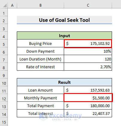
- Hence, the Goal Seek Status dialog box will appear with a solution associated with the target value of 1500.
- Click OK to keep the solved output.
- To ignore the solution, hit Cancel.

- After pressing OK, you’ll see the desired change in the buying price.
- This way, you can perform a reverse what-if analysis with Goal Seek.
2. Use Excel Solver Tool to Do Reverse What-If Analysis
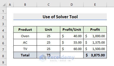
However, for multiple constraints, we have to use the Excel Solver tool. The Solver tool is a data analysis add-in that can determine the maximum or minimum output by considering all the constraints. To elaborate on reverse what-if analysis with this tool, we’ll use the below dataset. It contains Product, Unit, Total Profit, etc. Here, we want to Maximize the Total Profit by varying the units sold for different products. And the constraints are:
Total Units to be sold = 250
Minimum Units for Oven = 45
Minimum Units for AC = 40
Maximum Unit for TV = 35
Therefore, learn the following steps to carry out the operation.
STEPS:
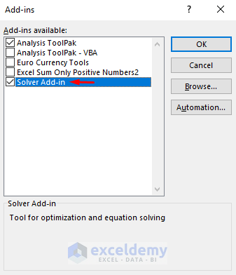
- Firstly, to add the Solver tool to the Data Analysis ribbon, go to File > Options.
- In the Excel Options dialog box, click Go for Excel Add-ins in the Add-ins tab.

- Check the box for Solver Add-in.
- Then, press OK.
- Subsequently, select Data > Analysis > Solver.
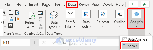
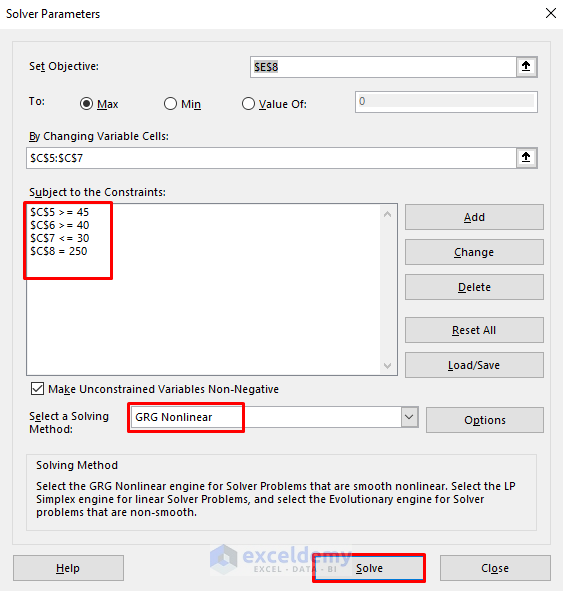
- Consequently, the Solver Parameters box will emerge.
- There, choose cell E8 for Set Objective.
- After that, select Max.
- Input C5:C7 or select the range in the By Changing Variable Cells box.
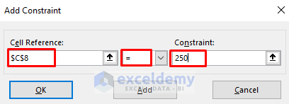
- Now, to add the constraints, press Add.

- There, choose Cell Reference > C8 for total units.
- Select = operator.
- Constraint > 250.
- Again press Add.
- Select Cell Reference > C5 for Oven.
- Select >= operator.
- Constraint > 45.
- Afterward, click Add, and in this way, input all the constraints.

- Finally, you’ll see all the required conditions in the dialog box.
- Next, choose the default GRG Nonlinear as the solving method.
- After that, press Solve to find the solution.
- Thus, it’ll return a dialog box after solving the math.
- Then, press OK to keep the solution or Cancel to drop it.

- At last, you’ll see the maximum profit.
- In such a way, we can perform a reverse what-if analysis.

Download Practice Workbook
Download the following workbook to practice by yourself.
Conclusion
Henceforth, you will be able to do Reverse What-If Analysis in Excel using the above-described approaches. Keep using them and let us know if you have more ways to do the task. Don’t forget to drop comments, suggestions, or queries if you have any in the comment section below.
Related Articles
- How to Use Goal Seek in Excel
- How to Do What-If Analysis Using Goal Seek in Excel
- How to Use Goal Seek to Find an Input Value
- How to Automate Goal Seek in Excel
- Excel Macro to Goal Seek for Multiple Cells
<< Go Back to Goal Seek in Excel | What-If Analysis in Excel | Learn Excel
Get FREE Advanced Excel Exercises with Solutions!
