How to Use Goal Seek in Excel (5 Examples)

What Is Goal Seek in Excel

Goal Seek is a feature of the What-If Analysis Command in Excel. This feature helps to find a specific input value for the desired output from a formula. You can solve many real-life problems by using this feature. This feature uses the trial and error method to back-calculate the input value.

Parameters of Goal Seek

3 parameters in the Goal Seek dialog box must be specified to get the result. They are:

1. Set cell: In the Set cell parameter, you must select the cell containing the formula. This is the cell where you want to find the targeted value.

2. To value: In this parameter, you must enter the value you want as the formula’s output.

3. By changing cell: In this parameter, select the cell where you want to change or find the input value.

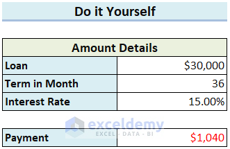
Example 1 – Solving a Mortgage Problem in Excel by Using Goal Seek

Steps:

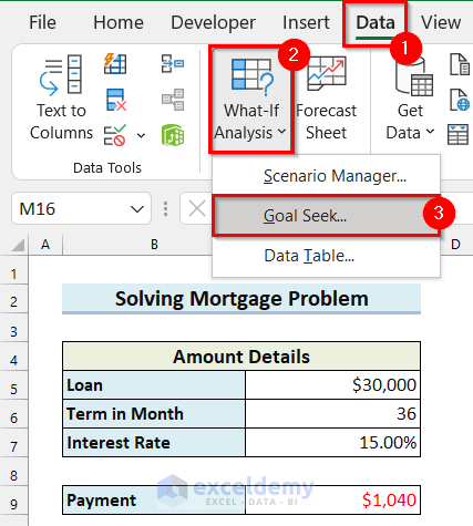
Go to the Data tab.
Select What-If Analysis.

A drop-down menu will appear.

Select Goal Seek from the drop-down menu.

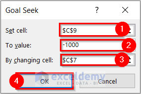
Selecting What-If Analysis Command to use Goal Seek in Excel

A dialog box named Goal Seek will appear.

Select the Set cell. Here, I selected cell C9 because it contains the payment formula.
Enter To value. Here, I wrote -1000 because the maximum Payment is limited to $1’000. And, as you are making a Payment the sign is negative.
Select By changing cell. Here, I selected cell C7 because this cell contains the Interest Rate.
Select OK.

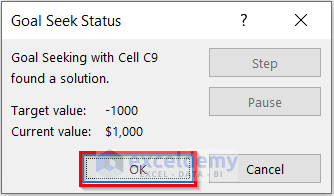
Another dialog box named Goal Seek Status will appear. This dialog box displays the Target value and the current value.

Select OK.

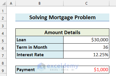
You can see that I have found the highest annual Interest Rate you can tolerate if your maximum monthly Payment limit is $1,000.

Example 2 – Using Goal Seek to Find Unknown Value in Excel

Steps:

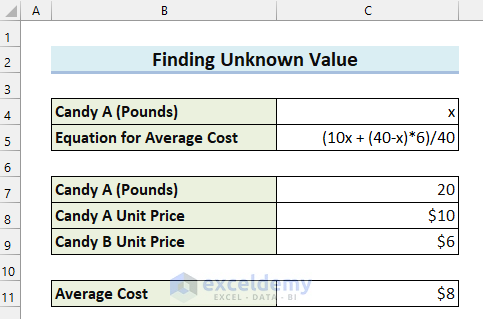
Select the cell where you want to calculate the Average Cost. Here, I selected cell C11.
In cell C11, enter the following formula:

=(C7*C8+(40-C7)*C9)/40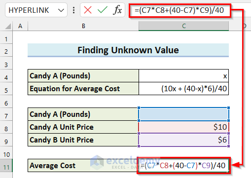

Inserting Formula to Use Goal Seek in Excel

Here, the formula will subtract the value in cell C7 from 40 and then multiply it by the value in cell C9. Then, the value in cell C7 will be multiplied by the value in cell C7. Both of these values will now be summed to get the total cost. Then, the formula will divide the result by 40 and return the Average Cost.

Press ENTER to get the result.

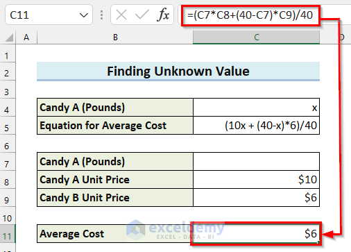
The Average Cost is not showing the right value as you have not entered any value in cell C7 yet. Here, I will explain how you can use the Goal Seek feature in Excel to find out the pounds of Candy A you need to buy to get an Average Cost of $8.

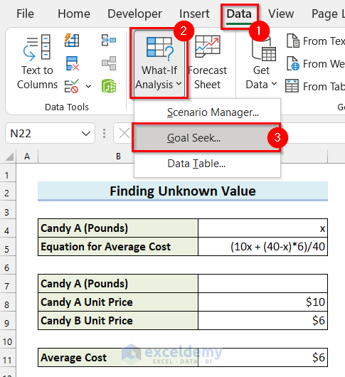
Go to the Data tab.
Select What-If Analysis.

A drop-down menu will appear.

Select Goal Seek from the drop-down menu.

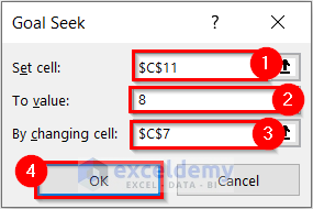
The Goal Seek dialog box will appear.

Select the Set cell. I selected cell C11 because this cell contains the formula for the Average Cost.
Enter To value. Here, I wrote 8 because the expected Average Cost is $8.
Select By changing cell. I selected cell C7 because this cell contains Candy A (Pounds).
Select OK.

Goal Seek Dialog Box in Excel

Another dialog box named Goal Seek Status will appear. This dialog box displays the Target value and the Currant value.

Select OK.

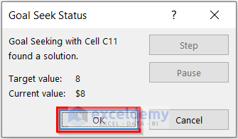
You can see that I have found how many Pounds of Candy A you will need to buy to make the average cost $8.

Example 3 – Applying Goal Seek to Find Breakeven Point

Steps:

Select the cell where you want to calculate the Profit.
Enter the following formula in the selected cell:

=C9*C10-C5-C6-C7*C8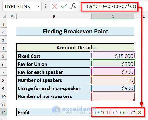

Formula for Profit to Use Goal Seek in Excel

Here, the value in cell C9 is multiplied by the value in cell C10. Then, the value in cell C5 and cell C6 is subtracted from the result. Then, the value in cell C7 is multiplied by the value in cell C8, which is subtracted from the previous result and returns the profit.

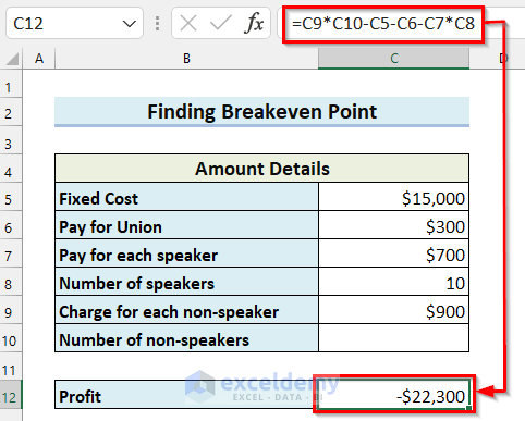
Press ENTER to get the Profit.

The Profit is -$22,300 because you do not have any gross income yet as you have not entered the Number of non-speaker.

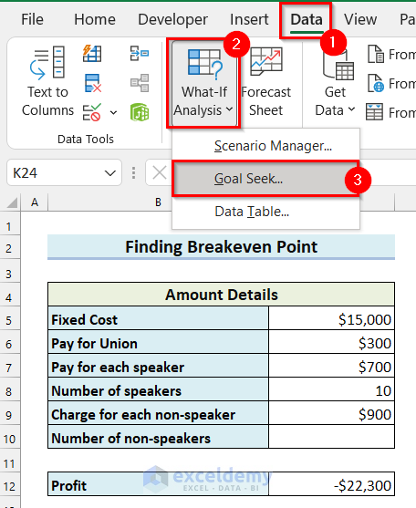
Go to the Data tab.
Select What-If Analysis.

A drop-down menu will appear.

Select Goal Seek from the drop-down menu.

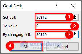
The Goal Seek dialog box will appear.

Select the Set cell. I selected cell C12 because this cell contains the formula for the Profit.
Enter To value. I wrote 0 because the Profit is 0 at the breakeven point.
Select By changing cell. I selected cell C10 because this cell contains the Number of non-speakers.
Select OK.

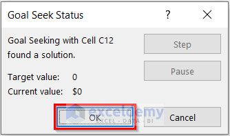
Another dialog box named Goal Seek Status will appear. This dialog box displays the Target value and the Currant value.

Select OK.

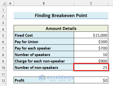
I got the Number of non-speakers needed for you to reach the breakeven point by using Goal Seek and, it is 25.

Example 4 – Solving an Equation in Excel by Using Goal Seek

Steps:

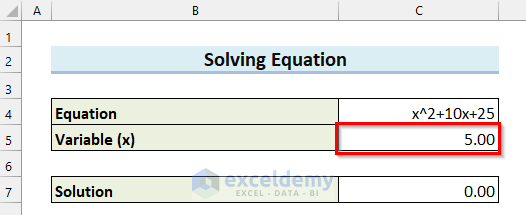
Select the cell where you want the Solution of the equation. Here, I selected cell C7.
In cell C7, enter the following formula:

=C5^2-10*C5+25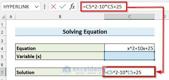

Here, the formula will raise the value in cell C5, the x, to the power of 2. Then, multiply the value in cell C5 by 10 and then subtract it from the previous result. After that, it will add 25 with the result and return the Solution of the equation.

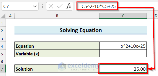
Press ENTER to get the result.

The result is 25 as I have not entered any value for the Variable (x).

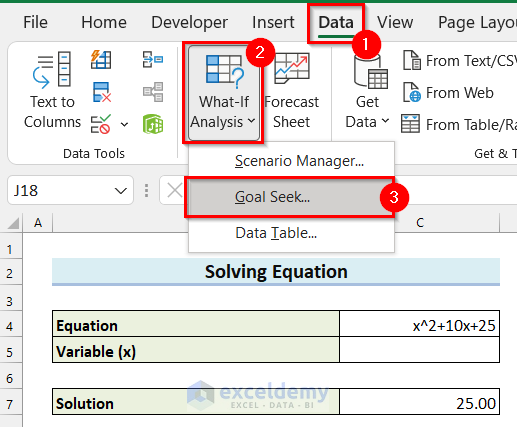
Go to the Data tab.
Select What-If Analysis.

A drop-down menu will appear.

Select Goal Seek from the drop-down menu.

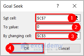
The Goal Seek dialog box will appear.

Select the Set cell. Here, I selected cell C7 because this cell contains the formula for the Solution of the equation.
Enter To value. I wrote 0 because the Solution is 0 in the given equation.
Select By changing cell. I selected cell C5 because this cell contains the Variable (x).
Select OK.

Another dialog box named Goal Seek Status will appear. This dialog box displays the Target value and the Currant value.

Select OK.

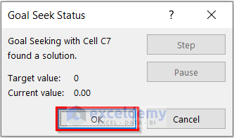
You can see that I have found the value of the Variable (x) by using the Goal Seek feature in Excel.

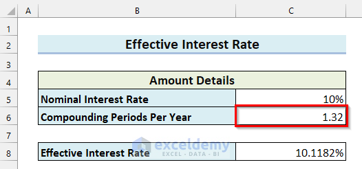
Example 5 – Using Goal Seek in Excel for Effective Interest Rate

Steps:

Select the cell where you want to calculate the Effective Interest Rate. Here, I selected cell C8.
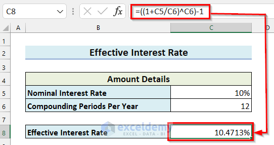
In cell C8, enter the following formula:

=((1+C5/C6)^C6)-1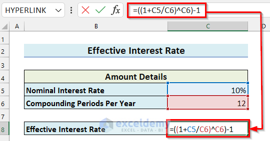

Using Goal Seek in Excel for Effective Interest Rate

Here, I divided the value in cell C5 by the value in cell C6 and then added 1 with the result. Then, the result is the power of the value in cell C6. After that, I subtracted 1 from the result, and the formula will return the Effective Interest Rate.

Press ENTER to get the result.

I will use the Goal Seek feature to find the Compounding Periods Per Year needed for the Effective Interest Rate to be 10.2%.

Go to the Data tab.
Select What-If Analysis.

A drop-down menu will appear.

Select Goal Seek from the drop-down menu.

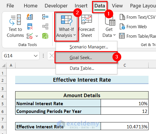
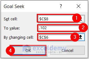
The Goal Seek dialog box will appear.

Select the Set cell. I selected cell C8 because this cell contains the formula for the Effective Interest Rate.
Enter To value. I wrote .102 because the expected Effective Interest Rate is 10.2%.
Select By changing cell. I selected cell C6 because this cell contains the Compounding Periods Per Year.
Select OK.

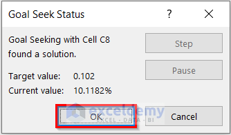
Another dialog box named Goal Seek Status will appear. This dialog box displays the Target value and the Current value. The Current Value does not match exactly with the Target Value, but it is close, and I am satisfied with it.

Select OK.

I have found the Compounding Periods Per Year for the desired Effective Interest Rate.

How to Use Goal Seek in Excel For Multiple Cells

Steps:

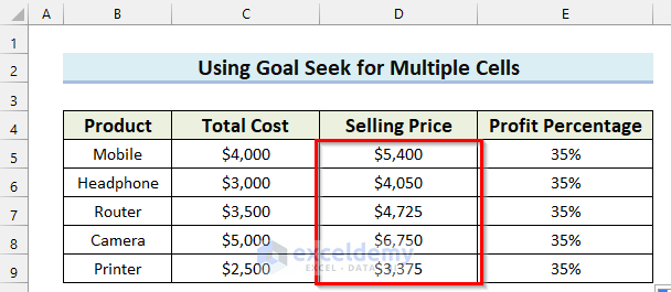
Select the cell where you want to calculate the Profit Percentage. Here, I selected cell E5.
In cell E5, enter the following formula:

=((D5-C5)/C5)*100%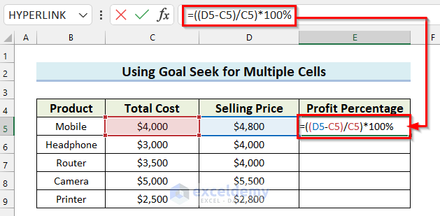

Here, I subtracted the value in cell C5 which is the Total Cost from the value in cell D5 which is the Selling Price. And, then divided the result by the value in cell C5. Then, I multiplied the result by 100% and now the formula will return the Profit Percentage.

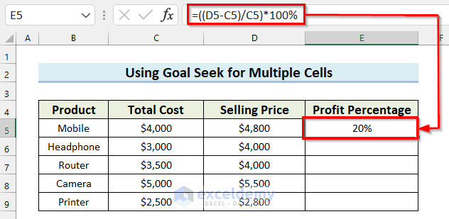
Press ENTER to get the result.

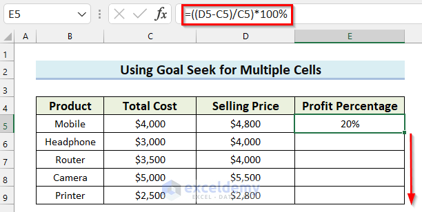
Drag the Fill Handle to copy the formula to the other cells.

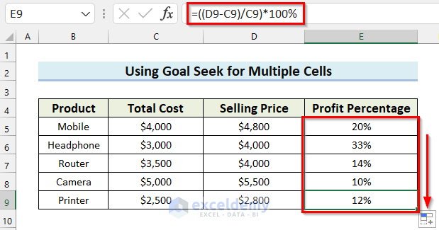
You can see that I have copied the formula and calculated the profit percentage for each product.

I will show you how to use Excel VBA to use Goal Seek for multiple cells. Here, I will find out the Selling Price for every Product if I want the Profit Percentage to be 35%.

Go to the Developer tab.
Select Visual Basic.

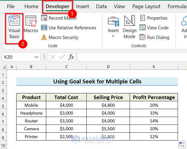
Opening Visual Basic Window to Use Goal Seek in Excel for Multiple Cells

The Visual Basic editor window will open.

Select the Insert tab.
Select Module.

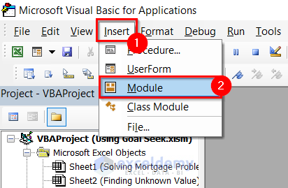
Inserting Module to Write VBA Code to Use Goal Seek in Excel

A module will open.

Enter the following code in that module:

Sub Goal_Seek_Multi_Cells()
For row_no = 5 To 9
Worksheets("Goal Seek for Multiple Cells").Cells(row_no, "E").GoalSeek Goal:=0.35, _
ChangingCell:=Worksheets("Goal Seek for Multiple Cells").Cells(row_no, "D")
Next row_no
End Sub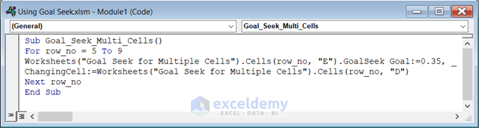

VBA Code for Goal Seek in Excel for Multiple Cells

Code Breakdown

Here, I created a Sub Procedure named Goal_Seek_Multi_Cells.
Then, I used a For Next Loop to go through multiple cells in a column.
Next, I used the GoalSeek method and set the Goal and ChangingCell according to the need. The GoalSeek method will change the value in ChangingCell to achieve the Goal in the selected cell.
Finally, I ended the Sub Procedure.

Save the code and go back to the worksheet.
Go to the Developer tab.
Select Macros.

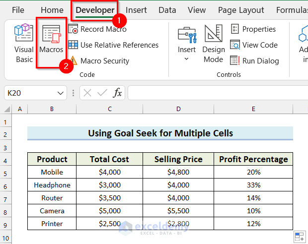
A dialog box named Macro will appear.

Select the Macro name.
Select Run.

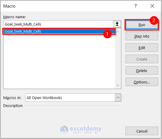
Running Macros to Use Goal Seek for Multiple Cells in Excel

You will see the Selling Price of every product has changed accordingly to get a Profit Percentage of 35%.

Read More: How to Automate Goal Seek in Excel

Goal Seek Precision in Excel

Steps:

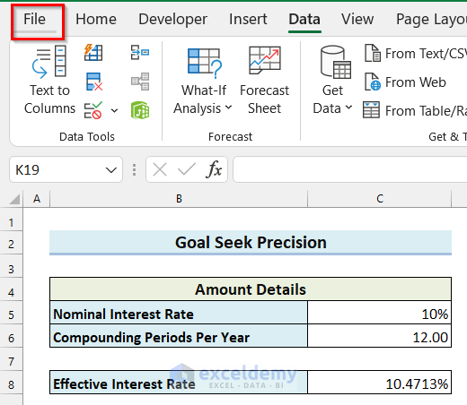
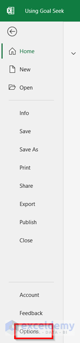
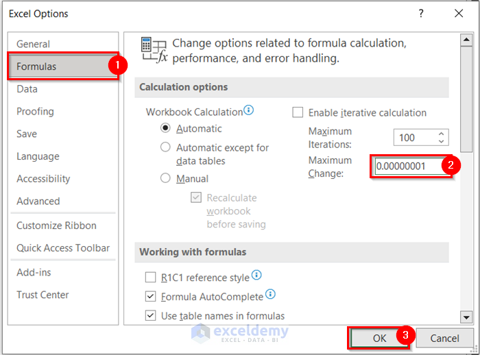
Go to the File tab.

Goal Seek Precision

Select Options.

A dialog box named Excel Options will appear.

Go to the Formulas tab.
Decrease the value for Maximum Change to get a more precise result.
Select OK.

Go back to the worksheet.

Go to the Data tab.
Select What-If Analysis.
Select Goal Seek.

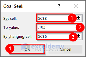
The Goal Seek dialog box will appear.

Select the Set cell. I selected cell C8 because this cell contains the formula for the Effective Interest Rate.
Enter To value. I wrote .102 because the expected Effective Interest Rate is 10.2%.
Select By changing cell. I selected cell C6 because this cell contains the Compounding Periods Per Year.
Select OK.

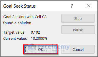
Another dialog box named Goal Seek Status will appear. This dialog box displays the Target value and the Current value. Here, the Current Value matches the Target Value, and I have achieved a more precise result.

Select OK.

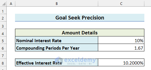
You can see that I have found the Compounding Periods Per Year for my desired Effective Interest Rate.

Things to Remember

It should be noted that the cell you are selecting for By changing the cell parameter must contain a value. If the cell contains a formula, then you will get an error.
Whenever working with VBA, you must save the Excel file as an Excel Macro-Enabled Workbook. Otherwise, the macros won’t work.