What is the Reference (#REF!) Error in Excel?
The reference (#REF!) error is usually displayed when a cell referred to in the Excel formula is not valid.
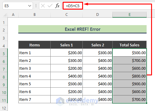
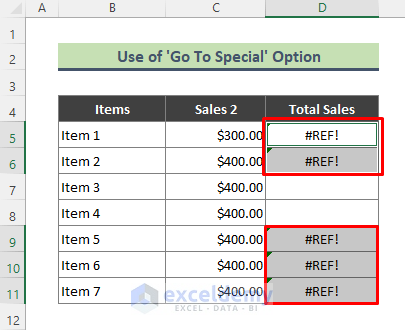
The dataset showcases sales data. The total sales was calculated using a formula. Here, the summation formula used C5 and D5 as reference.
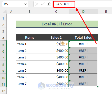
If column C is deleted, #REF! errors will be displayed.
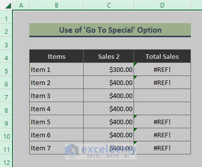
Method 1 – Using the ‘Go To Special’ Option to Find Reference (#REF!) Errors
Steps:
- Select the entire worksheet that contains reference (#REF!) errors.
- Press Ctrl + G to open the ‘Go To’ dialog box.
- Click Special.

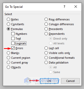
- In the ‘Go To Special’ dialog box, select Formulas.
- Check Errors.
- Click OK.
- All cells containing #REF! errors will be displayed.
Note:
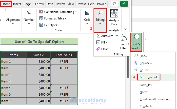
- You can also open the Go To Special dialog box by following the path: Home > Editing group > Find & Select > Go To Special.
Read More: How to Remove Error in Excel
Method 2 – Using the Excel Find Option to Search Reference (#REF!) Errors
Steps:
- Select the entire worksheet.
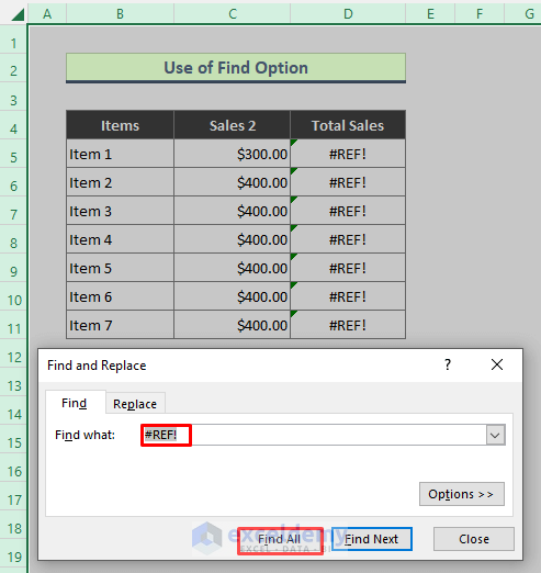
- Press Ctrl + F to open the Find and Replace dialog box.
- Enter #REF! in Find what and click Find All.
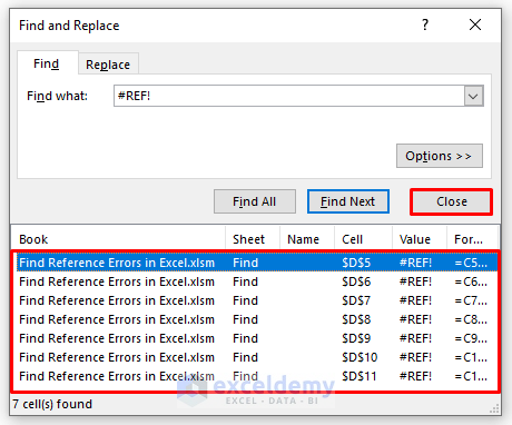
- You will see a list indicating cells with #REF! errors.
- Click Close.
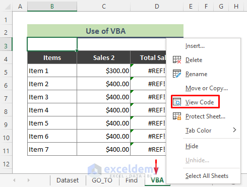
Method 3 – Using Excel VBA to Find Reference (#REF!) Errors
Steps:
- Go to the worksheet where you want to locate the reference error, right-click the sheet name, and press View Code to display the VBA window.
- Enter the code in the Module.
- Run the code by pressing F5.
Sub Get_REF()

Dim a As Range
For Each a In ActiveSheet.UsedRange
    If a.HasFormula = True And InStr(1, a.Formula, "#REF!", 1) > 1 Then MsgBox a.Address
Next a

End Sub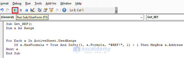
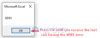
- A message box will display the cell reference that has the #REF! errors.
- Click OK until you get the last cell reference.
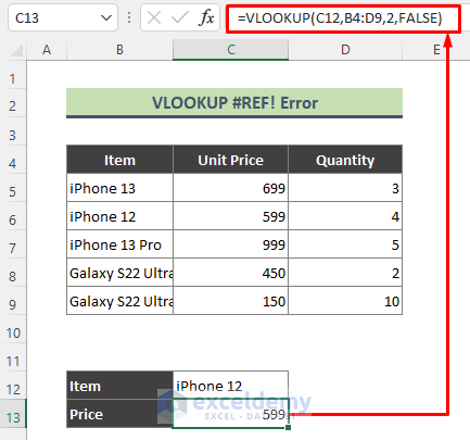
VLOOKUP Reference (#REF!) Errors in Excel
The formula below returns #REF! because the column index number is entered as 4. The lookup table has 3 columns only.
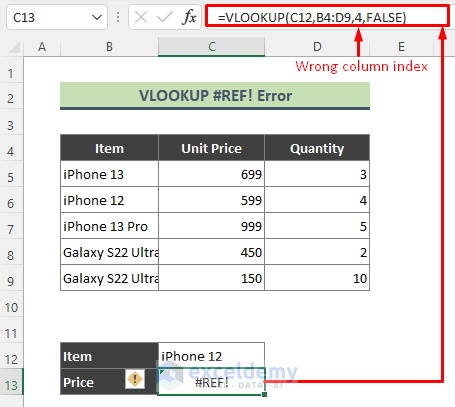
Enter 2, instead of 4, to fix the error.
Other Possible Reasons for Excel Reference (#REF!) Errors
- Macro Issues: When the cell above the function is in row 1, #REF errors may be displayed. Edit the macro.
- Object Linking and Embedding (OLE) Issues: When an OLE link returns #REF errors, run the program that the link is referencing.
- Dynamic Data Exchange (DDE) Issues: While using DDE reference the right topic. If an error occurs, in Excel Trust Center Settings, review the external content settings.
Avoid Reference (#REF!) Errors in Excel
- Modify your formula so that the deletion of columns/ row/ sheets won’t affect it. Use a range of formulas to calculate the summation ‘=SUM(C5:D5)’ instead of a simple summation formula (=C5+D5).
- You may need to copy formulas to other locations. Avoid using relative references. Instead, use absolute references in formulas.
Download Practice Workbook
Download the practice workbook.
Related Articles
- How to Correct a Spill (#SPILL!) Error in Excel
- [Fixed!] ‘There Isn’t Enough Memory’ Error in Excel
- [Fixed] Excel Print Error Not Enough Memory
<< Go Back To Excel Formula Errors | Errors in Excel | Learn Excel
Get FREE Advanced Excel Exercises with Solutions!
