Multiple Groups from the Same Data Source

If you create more than one pivot table from the same data source, and you have created a group of items in a pivot table, this group will automatically be copied in another pivot table. All the other pivot tables will use this same group. Sometimes, this is exactly what you want. Other times, it’s not at all what you want. For example, you may need two pivot table reports: one pivot table will summarize data by month and year, and another pivot table will summarize the data by quarter and year. See the following figure.

All the pivot tables use the same pivot table “cache”. This is why grouping in a pivot table affects other pivot tables. This is unfortunate for us that, we can’t directly force a pivot table to use a new cache. But we can use a trick to force Excel into using a new cache. The trick is we shall give multiple range names to the source data.

For example, we shall name our source data range Table1, and then we shall give the same data range a second name: Table2. You can use the Name box to name a range, it is the easiest way. Select the data range, name in the Name box, and press Enter. Then, with the data range still selected, enter a different name in the Name box, and press Enter. Only the first name will be displayed in the Name box if you select the data range, but you can verify that both names exist for this data range by choosing Formulas ➪ Define Names ➪ Name Manager.

When you will create your first pivot table, you will specify Table1 as the Table/Range. When you will create your second pivot table, you will specify Table2 as the Table/Range. Each pivot table will now use a separate cache. So you can create independent groups in one pivot table, that will not affect the groupings in other pivot tables.

An Example

Take a look at the following screenshot. There are 730 rows in this data range and we shall create two pivot tables but each pivot table will have independent groupings. The first pivot table will be grouped by month and by year, and the second pivot table will be grouped by quarter and by year.

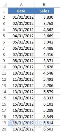
Sales day by date. This table has 730 rows covering data between 1st January 2012 and 31rd 2013

Download this sample file where we have done this example

Creating a pivot table from Table1

Step 1:

Select the data range A1: B731 and enter Table1 in the Name box, and press Enter. Data range A1: B731 is now named Table1.

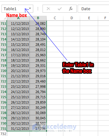
Enter Table1 in the Name box.

Step 2:

Then, with the data range still selected, enter a different name Table2 in the Name box, and press Enter. Only the first name will be displayed in the Name box if you select the data range, but you can verify that both names exist for this data range by choosing Formulas ➪ Define Names ➪ Name Manager.

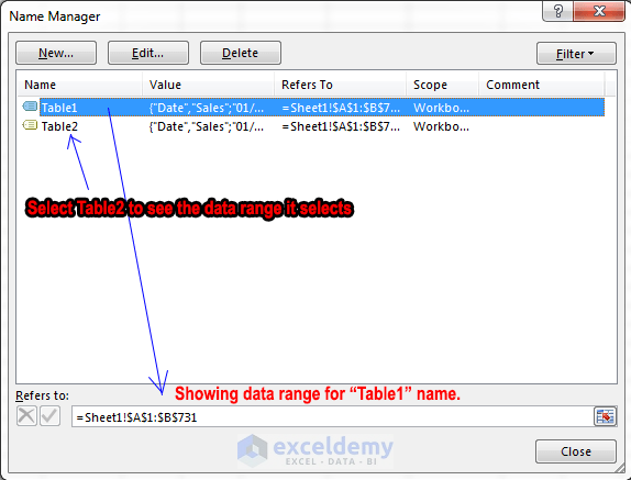
Choose Formulas ➪ Define Names ➪ Name Manager to see the names of data range A1: B731

Step 3:

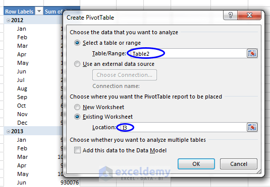
Now select any cell in the data range A1: B731 and choose INSERT ⇒ Tables ⇒ PivotTable. Create PivotTable dialog box will appear. Enter Table1 in the Table/ Range field and E3 in the Location field. The location field will be activated when you will choose Existing Worksheet radio button. Then click OK.

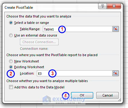
Choosing data range Table1 as the data source

Step 4:

After clicking OK in the Create PivotTable dialog box, a pivot table skeleton will be placed in the same worksheet in cell E3. Place Date field in the Rows area and Sales field in the Values area in the PivotTable Fields task pane. Right-click on any cell under the Row Labels column in the pivot table, a shortcut menu will appear, and choose Group from the options in the menu. A grouping dialog box will appear and choose Months and Years from the By list and click OK.

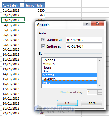
Select Months and Years from By list in the Grouping dialog box

You will get a pivot table like the one shown in the following figure.

Pivot Table created from Table1 data source.

Read More: How to Rename a Default Group Name in Pivot Table (2 Ways)

Creating the pivot table from Table2

Use the above steps to create a pivot table. Just use Table2 as Table/ Range in Create PivotTable dialog box and choose Quarters and Years from the By list in the Grouping dialog box.

Change in the Create PivotTable dialog box.

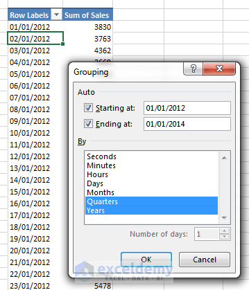
Change in the Grouping dialog box.

You will get two pivot tables as shown in the following screenshot.

Finally, we have got two pivot tables with different groupings.

Read More: How to Group Data in Pivot Table (3 Simple Methods)

Changing Data source of existing Pivot Table

You can also change the data source o the existing pivot table. You have to make sure that you have given your data source e different name. Then select the pivot table and choose PivotTable Tools ➪ Analyze ➪ Data ➪ Change Data Source. Change PivotTable Data Source dialog box will appear, type the new name that you gave to the range in the Table/ Range field. Thus you can create a new pivot cache for the existing pivot table. Observe the following figure.

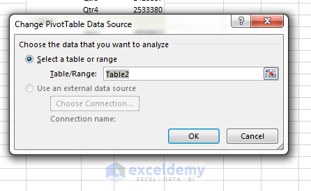
Change Pivot Table Data Source dialog box.

Happy Excelling 🙂

Related Articles

• [Fixed] Excel Pivot Table: Cannot Group That Selection (2 Easy Solutions)
• How to Use Excel Pivot Table to Group by Different Intervals (3 Methods)
• [Fixed] Excel Pivot Table Not Grouping Dates by Month
• How to Group Numbers in Excel Pivot Table (with Simple Steps)