Grouping means organizing data in a manner to view them at a glance. The Excel Pivot Table is a wonderful tool with a built-in feature for grouping. The Pivot Table can perform grouping based on date, text, number, etc. But here, we will discuss how to group numbers in an Excel Pivot Table with steps in detail.
Step 1: Inserting Data in Excel
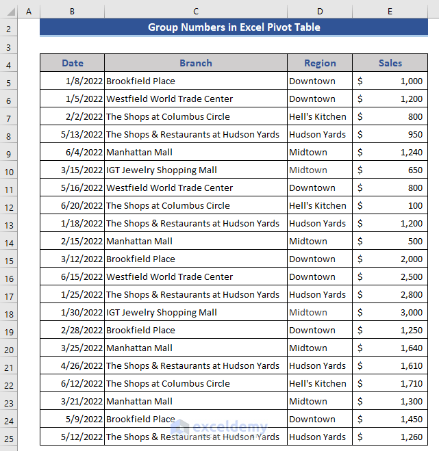
First, we need to insert data into the dataset. Our dataset consists of a super shop’s date, branch, region, and sales information. The super shop has several branches in different locations.
Step 2: Creating an Excel Pivot Table
In this step, we will create a PivotTable based on our dataset.
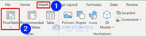
- First, go to the Insert tab.
- Click on the PivotTable option from the Tables group.
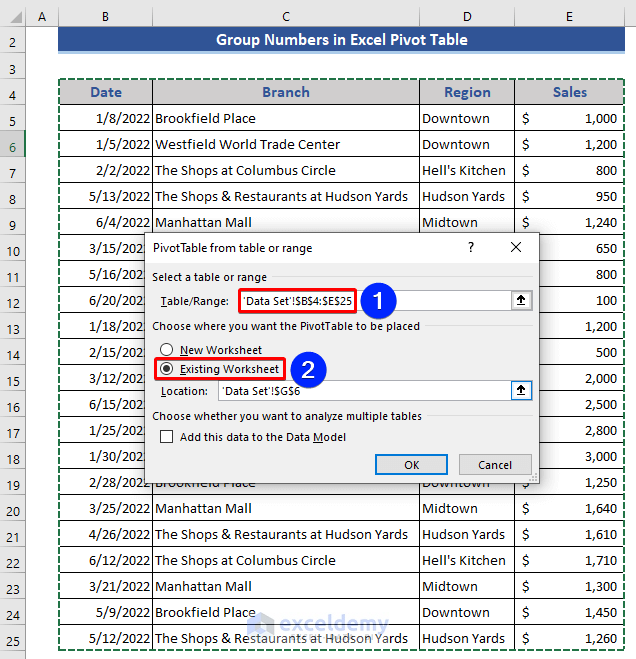
- The PivotTable from table or range window appears.
- In the Table/Range box, select the cells from the dataset.
- Choose the Existing Worksheet option.
- Finally, press the OK button.
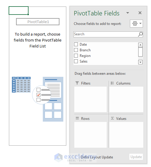
- Look a PivotTable appears in the dataset.
Step 3: Organizing Data in Pivot Table
In this step, we will organize our data in the PivotTable according to our desire.
- We insert Branch in the rows and Sales in the values section.
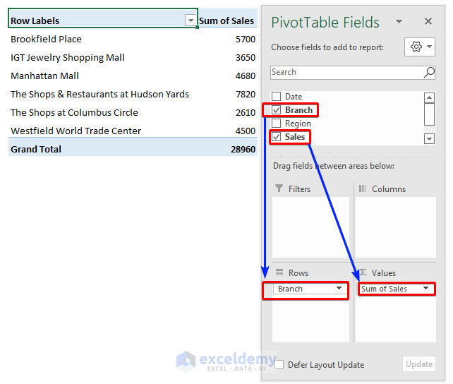
Sales data are shown against each branch.
- Now, insert Sales in the rows section.
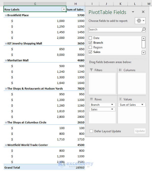
We want to know the occurrence number against each sales amount.
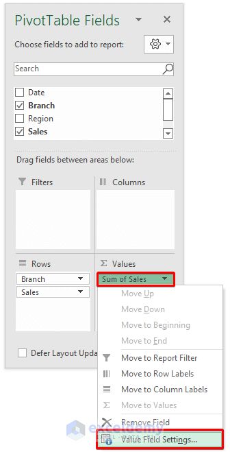
- Go to the values section.
- Click on the down arrow of the Sum of Sales option.
- Select Value Field Settings from the menu.
- The Value Filed Settings window appears.
- Choose the Count option from the Summarize Values By section.
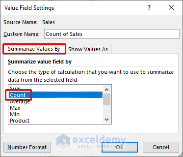
- Finally, press OK and see the PivotTable.
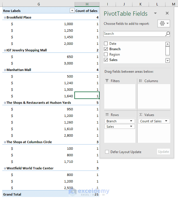
We can see the number of occurrences in the Count of Sales column.
Step 4: Grouping Numbers in Excel Pivot Table
In this step, we will group the numbers in the Excel PivotTable.
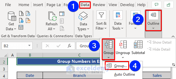
- Go to the Date tab.
- Choose Group from the Outline group.
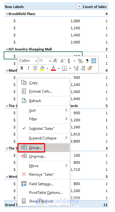
We have another alternative way to avail Group option.
- Click on any cell on the PivotTable. Now, press the right button of the mouse.
- Click on the Group option from the Context Menu.
- Now, the Grouping window appears.
- Here, the starting and the ending point is set by default.
- The By box indicates the difference.
- We set 250 You can set this value as per your need.
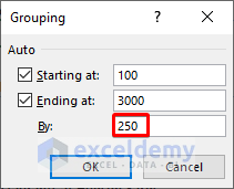
- Finally, press the OK button.
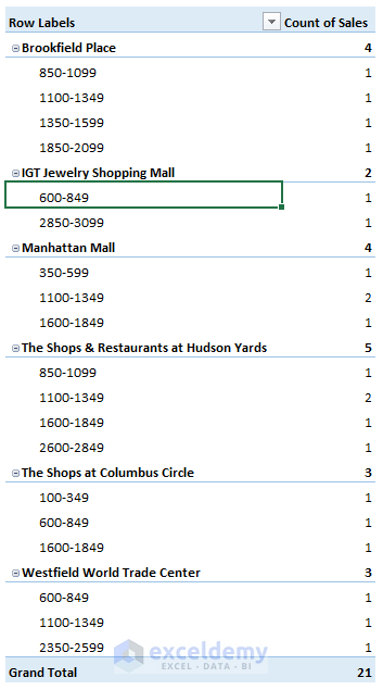
Here, Sales are grouped at a certain interval.
We also can change the data presentation as per our desire and data pattern.
Read More: How to Use Excel Pivot Table to Group by Different Intervals
Download Practice Workbook
Download this practice workbook to exercise while you are reading this article.
Conclusion
In this article, we described the steps of how to group numbers in an Excel Pivot Table. I hope this will satisfy your needs. Please, give your suggestions in the comment box.
Related Articles
- How to Make Group by Same Interval in Excel Pivot Table
- Pivot Table Custom Grouping
- How to Rename a Default Group Name in Pivot Table
- [Fixed] Excel Pivot Table: Cannot Group That Selection
- How to Group Rows in Excel Pivot Table
- How to Group Columns in Excel Pivot Table
<< Go Back to Group Pivot Table | Pivot Table in Excel | Learn Excel
Get FREE Advanced Excel Exercises with Solutions!
