How to Rename a Default Group Name in Pivot Table (2 Ways)

We’re going to use the following dataset which has 4 columns: Employee, Location, Group, and Sex.

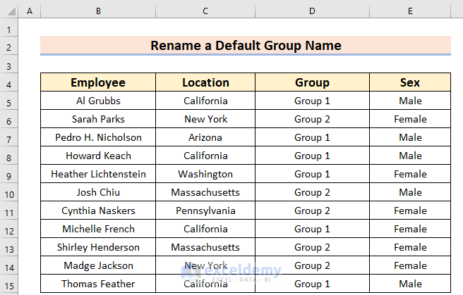
We’ll make a pivot table from it.

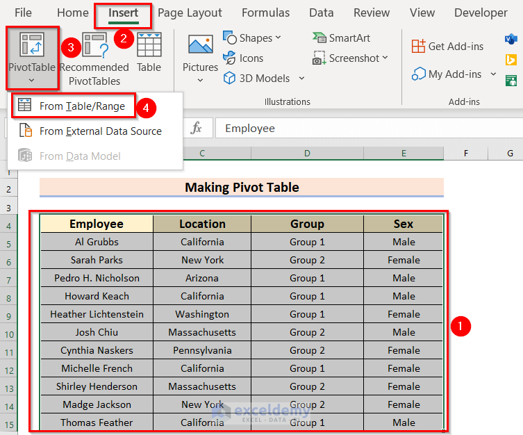
• Select the data range.
• From the Insert tab, go to PivotTable and choose the From Table/Range option.

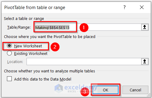
A dialog box named PivotTable from table or range will appear.

• Make sure that you have chosen the entire dataset.
• Mark the New Worksheet option.
• Press OK to get the result.

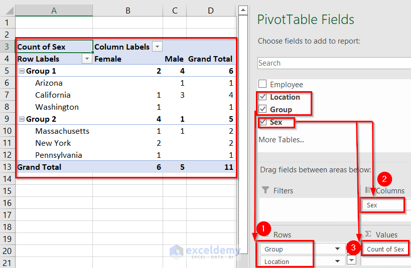
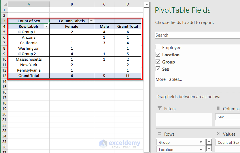
• Drag Group and Location to the Rows area.
• Drag Sex to the Columns and Values areas.

You will see the Pivot Table.

The formatted Pivot Table is given below.

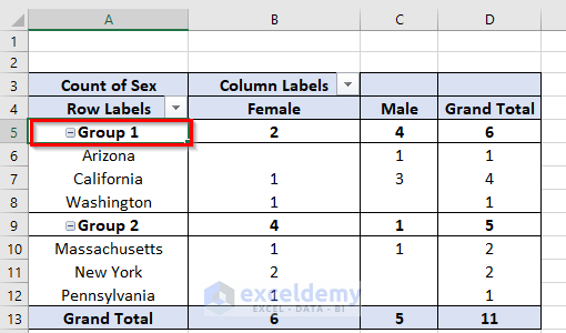
Method 1 – Use the F2 Button to Rename a Default Group Name in a Pivot Table

Steps:

• Select the data. We have selected the A5 cell.

• Press F2 from your keyboard.

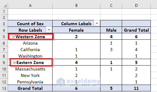
• Use Backspace to delete the existing group name, then enter a new group name. We have changed Group 1 into Western Zone and Group 2 into Eastern Zone.

Method 2 – Using the Formula Bar to Rename a Default Group Name in a Pivot Table

Steps:

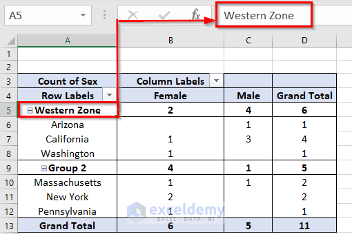
• Select the data. We have selected the A5 cell.
• Go to the Formula Bar.
• Press Backspace to remove the default name.

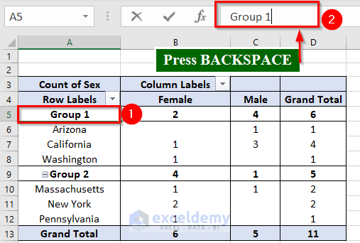
• Write down your preferred name in the Formula Bar. We have written “Western Zone” in the Formula Bar.
• Repeat for other cells as needed.

Read more: Pivot Table Custom Grouping

Download the Practice Workbook

Related Articles

• How to Group Columns in Excel Pivot Table
• How to Group Numbers in Excel Pivot Table
• [Fixed] Excel Pivot Table: Cannot Group That Selection
• How to Make Group by Same Interval in Excel Pivot Table

<< Go Back to Group Pivot Table | Pivot Table in Excel | Learn Excel