How to Group Columns in an Excel Pivot Table – 2 Methods

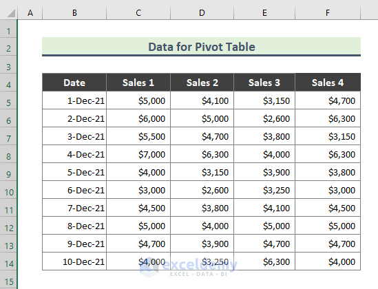
The dataset contains date-wise sales data from different stores.

Create a Pivot Table and group columns into Column Labels.

Method 1 – Creating a PivotTable and using the PivotChart Wizard to Group Columns in a Pivot Table

Steps:

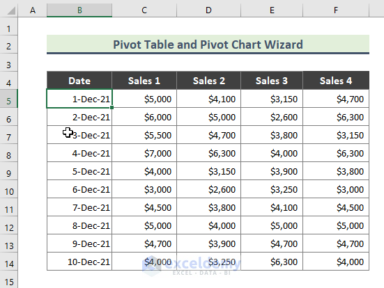
• Go to the source data sheet and press Alt + D + P.

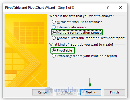
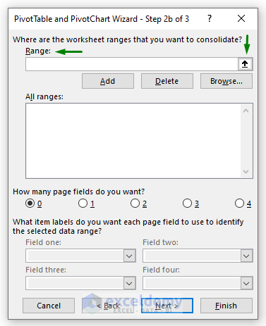
• The PivotTable and PivotChart Wizard will be displayed. Check Multiple consolidation ranges and PivotTable.
• Click Next.

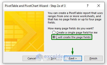
• Check I will create the page fields and click Next.

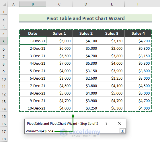
• Click the upward arrow in Range.

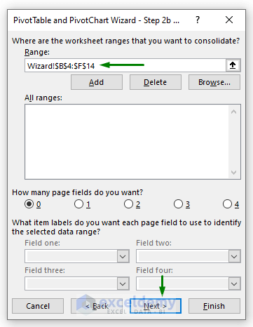
• Select the range for the Pivot Table.

• Click Next.

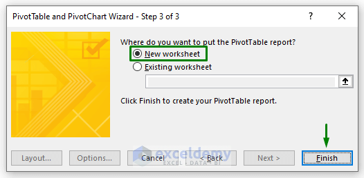
• Choose New Worksheet and click Finish.

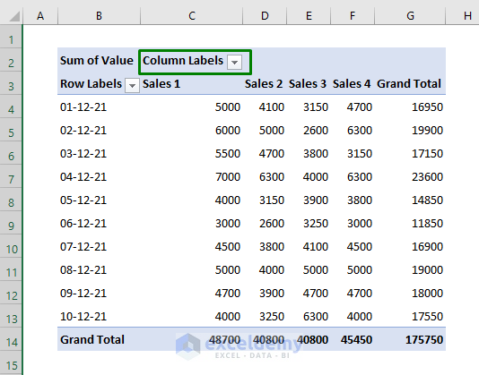
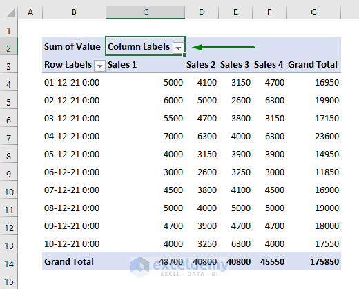
The Pivot Table is displayed. In the header of the Pivot Table, you will see the Column Labels drop-down icon.

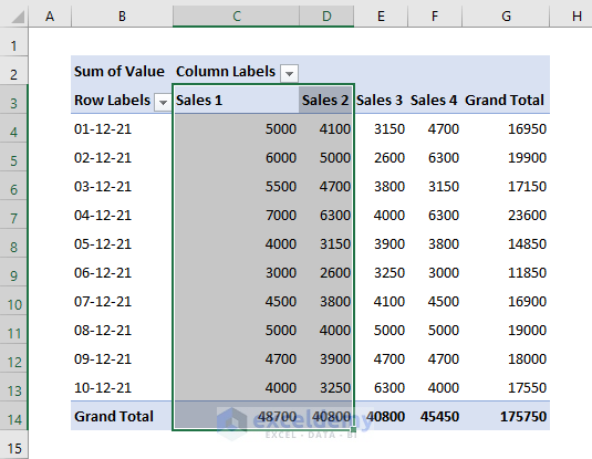
• To group data of Sales 1 and Sales 2 columns, select them first.

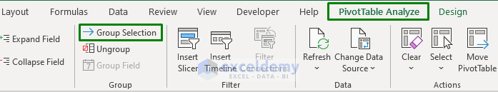
• Go to the PivotTable Analyze tab and select Group Selection.

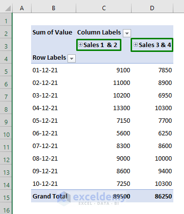
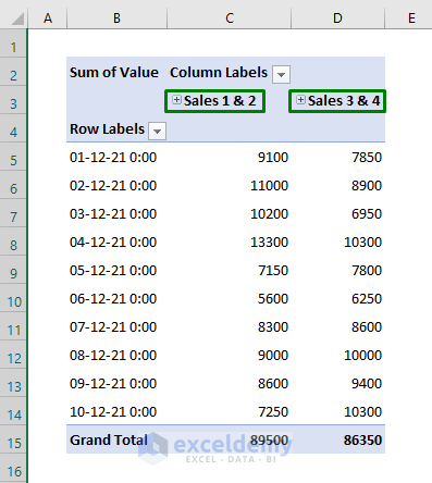
Sales 1 and Sales 2 Columns are grouped.

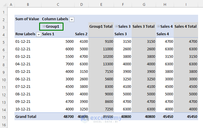
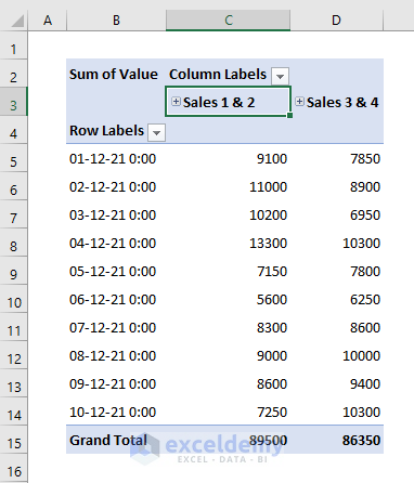
• You can rename the group.

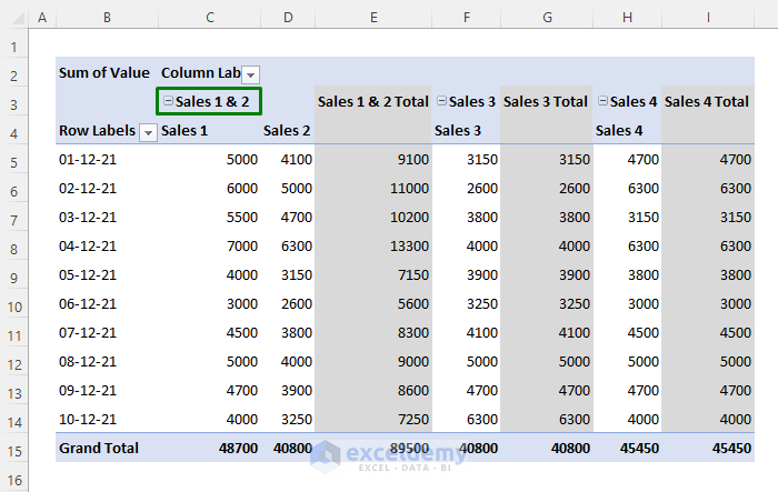
• You can group the columns Sales 3 and Sales 4 and get the following result:

Read More: How to Make Group by Same Interval in Excel Pivot Table

Method 2 – Using the Excel Power Query Editor to Group Columns in a Pivot Table

Steps:

• Go to the source dataset and press Ctrl + T. In the Create Table dialog box, check if the range of the table is correct, and click OK.

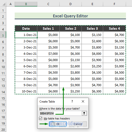
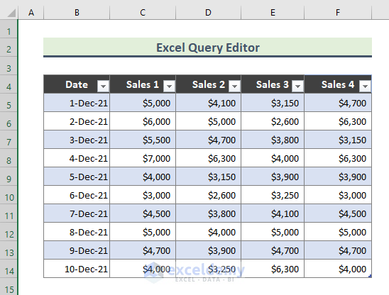
The table is created.

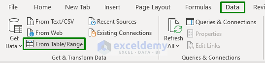
• Go to Data > From Table/Range.

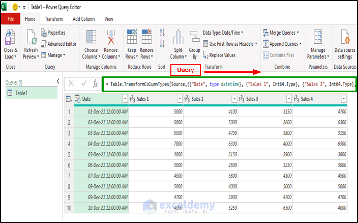
In the Power Query Editor window, by default, the table data will be displayed with an autogenerated query.

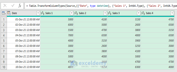
• Select the columns as shown below.

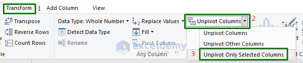
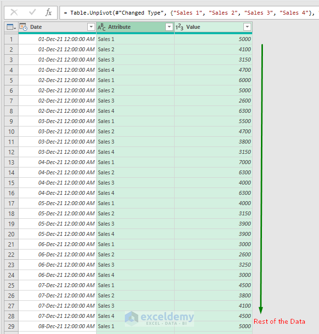
• In the Power Query Editor window, go to Transform > Unpivot Columns > Unpivot Only Selected Columns.

You will get the following data in the Power Query Editor.

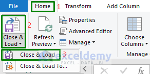
• In the Power Query Editor window, go to Home > Close & Load > Close & Load.

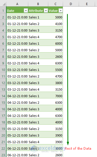
You will get the following table:

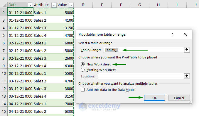
• Select the table and go to Table Design > Summarize with PivotTable.

• In the PivotTable from table or range dialog box, enter the Table/Range and select New Worksheet.
• Click OK.

A blank Pivot Table will be created.

Set the row/column values for the Pivot Table:

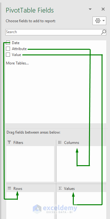
• Click the blank Pivot Table and go to PivotTable Fields.
• Drag Date to Rows, Attribute to Columns, and Value to Values.

• Group columns as described in Method 1.

Read More: Pivot Table Custom Grouping

Ungroup Columns in Excel Pivot Table

Steps:

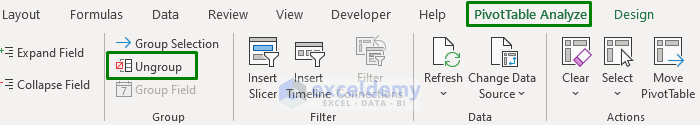
• Click the group name.

• Go to PivotTable Analyze > Ungroup.

Columns will be ungrouped.

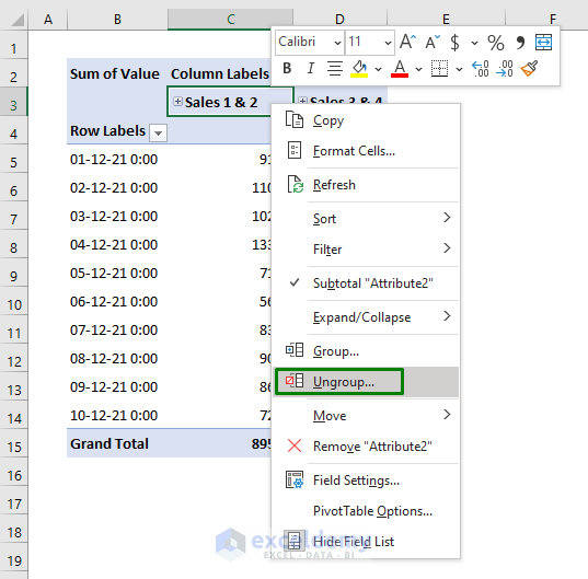
Note:

You can group/ungroup by right-clicking.

Download Practice Workbook

Download the practice workbook.

Related Articles

• How to Group Numbers in Excel Pivot Table
• How to Rename a Default Group Name in Pivot Table
• [Fixed] Excel Pivot Table: Cannot Group That Selection

<< Go Back to Group Pivot Table | Pivot Table in Excel | Learn Excel