This is the sample dataset.

Method 1 – Group by Time Intervals in Excel Pivot Tables
1.1 Group by Hour
Steps:
- Select data in your dataset.
- Click Insert > Pivot Table.

The Pivot table will automatically select the data range.
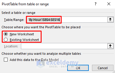
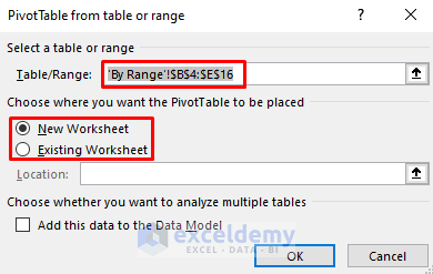
- Select the worksheet- New Worksheet/ Existing Worksheet.
- Click OK.
- In Pivot Table fields, drag Time to Rows and Sales to Values.

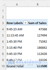
This is the output.
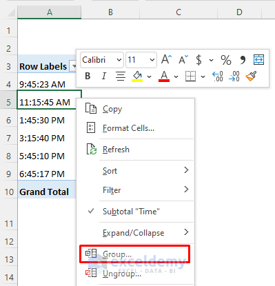
- Select any cell containing time.
- Right-click and select Group.
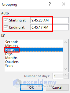
Start time and End time are automatically selected.
- Select Hours.
- Click OK.
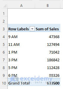
Sales are grouped by hours.
You can change the format of the Sum of values:
- Click the drop-down arrow in Sum of values.
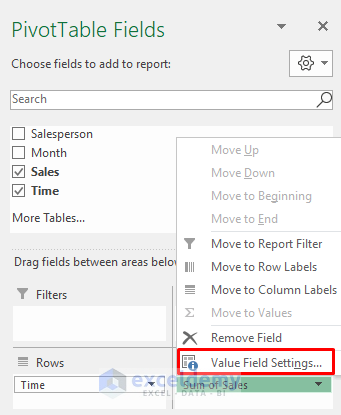
- Select Number Format.

- In Format Cells, click Currency in Category.
- Select the first option in Negative numbers.
- Click OK.

- Click OK.

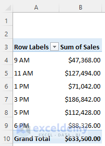
The selected format is applied:
1.2 Group by Custom Time Intervals
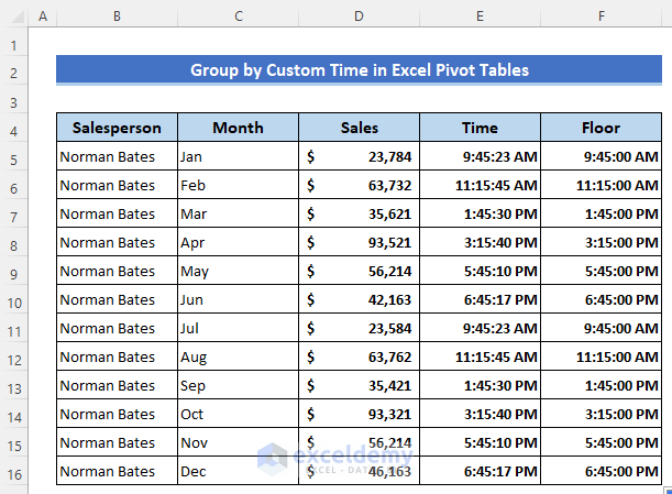
A new column was added: Floor.
Steps:
- Enter the following formula in F5.
=FLOOR(E5,"00:15")- Press Enter.

- Drag down the Fill Handle to copy the formula.

Rounded time is displayed.
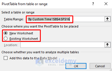
- Select data in the dataset.
- Click Insert > Pivot Table.
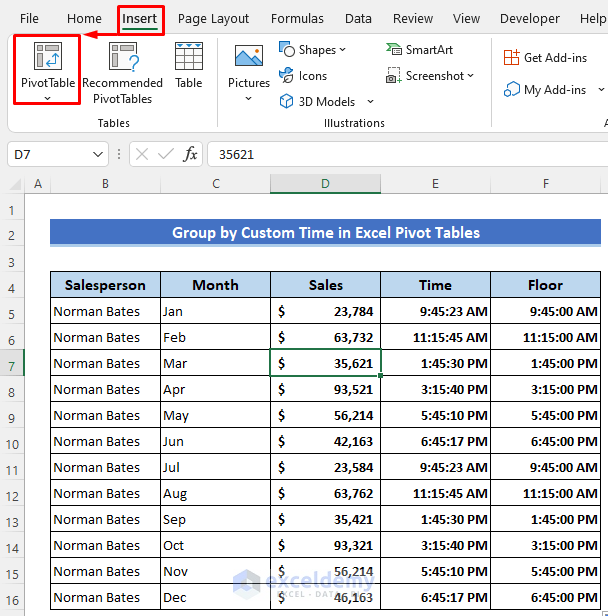
- Select the worksheet and click OK.
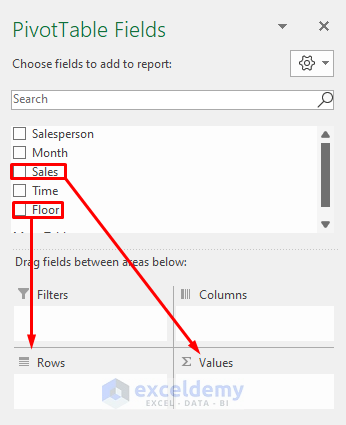
- In PivotTable Fields, drag Floor to Rows and Sales to Values.
This is the output.

Read more: Pivot Table Custom Grouping
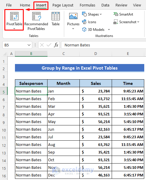
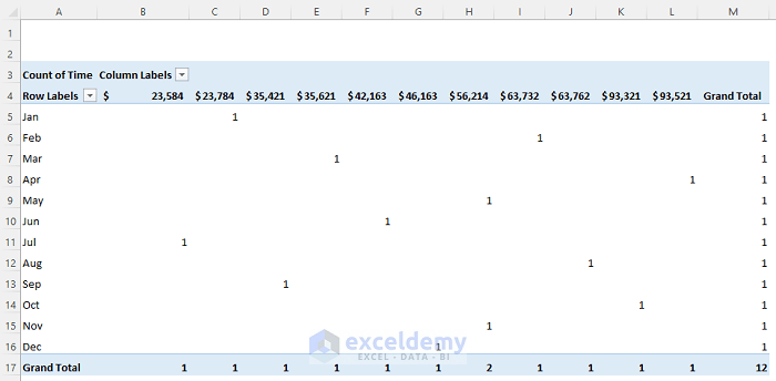
Method 2 – Group by Ranges in an Excel Pivot Table
Steps:
- Create Pivot Table by selecting any cell and clicking Insert > Pivot Table.
- Choose New worksheet and click OK.
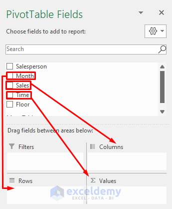
- Drag Month to Rows, Sales to Columns, and Time to Values.
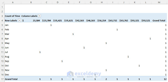
The Pivot Table is displayed:
- Click sales data.
- Right-click and select Group.
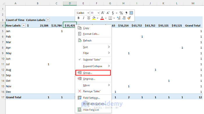
You can also click: PivotTable Analyze > Group Selection.

- In Grouping, choose the Starting at and Ending at values and enter the interval in By.
- Click OK.


Read more: How to Group Columns in Excel Pivot Table
How to Ungroup a Pivot table?
Steps:
- Select grouped data.
- Right-click.
- Click Ungroup.
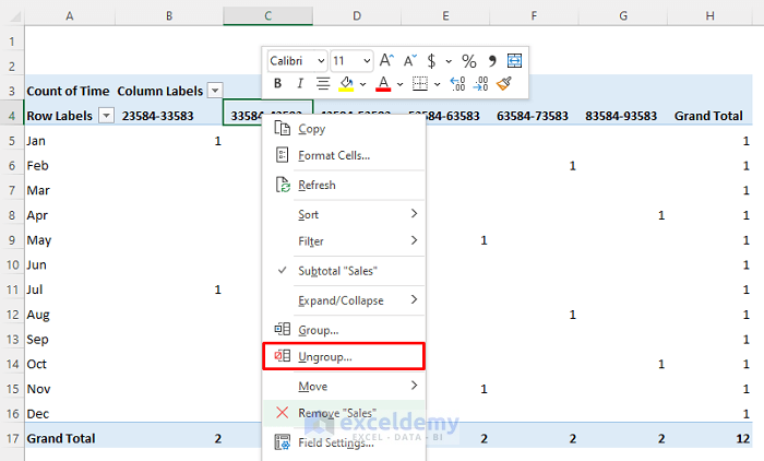
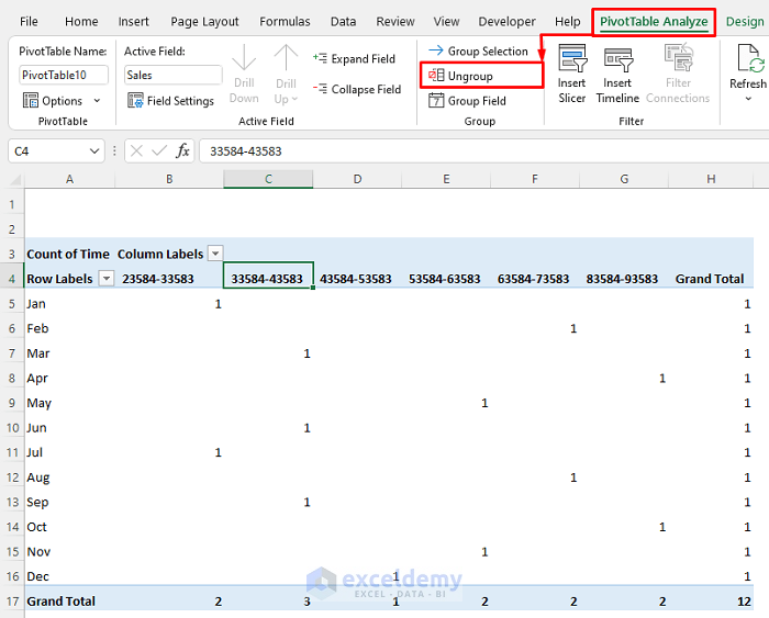
You can also click: PivotTable Analyze > Ungroup.
The Pivot Table is ungrouped.
Error and Solution
You may get the ‘Cannot group that selection’ error while grouping by the same interval.

Cells may contain text instead of numbers. Convert text to numbers before grouping.
Download Practice Workbook
Download the free Excel template.
Further Readings
<< Go Back to Group Pivot Table | Pivot Table in Excel | Learn Excel
Get FREE Advanced Excel Exercises with Solutions!
