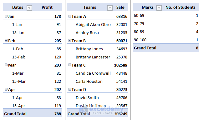
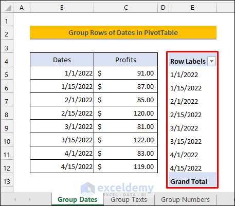
This article illustrates how to group rows in an Excel Pivot Table. Grouping values in a Pivot Table makes it more presentable and more easily understandable. The following picture highlights the results of grouping rows in the Pivot Table. Have a quick look through the article to learn how to do that.
1. Grouping Rows of Dates in Excel Pivot Table
Imagine you have the following dataset containing sales made on particular dates. Follow the steps below to create a PivotTable and then group the rows of dates in the table.

📌 Steps
- First, select anywhere in the dataset. Then, select the PivotTable icon from the Insert tab as shown in the following picture.

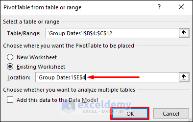
- Next, select the location for your PivotTable and then hit OK.
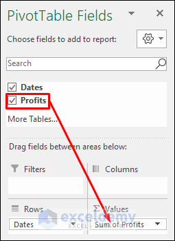
- Now, drag the Dates field into the Rows area as shown below.

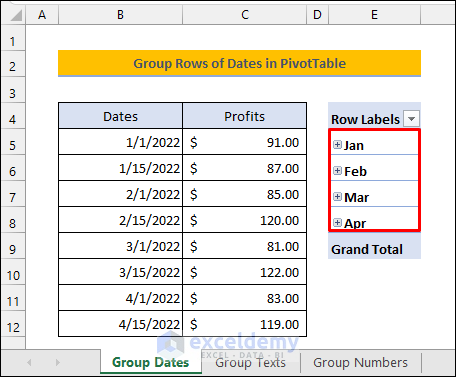
- As soon as you do that, Excel will group the dates automatically if you are using newer versions of Excel.
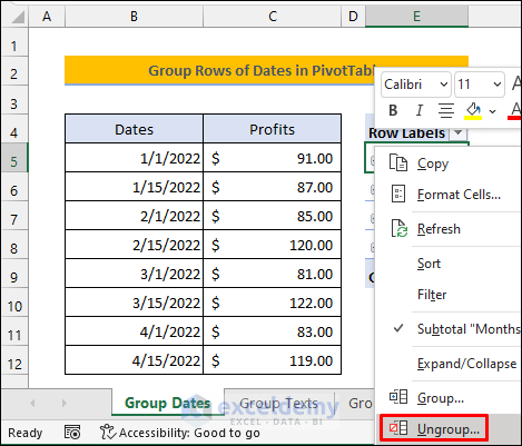
- After that, you can press CTRL+Z or select any group and right-click to ungroup them.
- Then, the PivotTable will look like the one below.
- Now, drag the Profits field in the Values area as shown in the picture below.
- After that, the table will be like the following one.

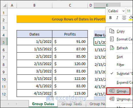
- Now, select any date in the PivotTable and then right-click. Then, select Group.
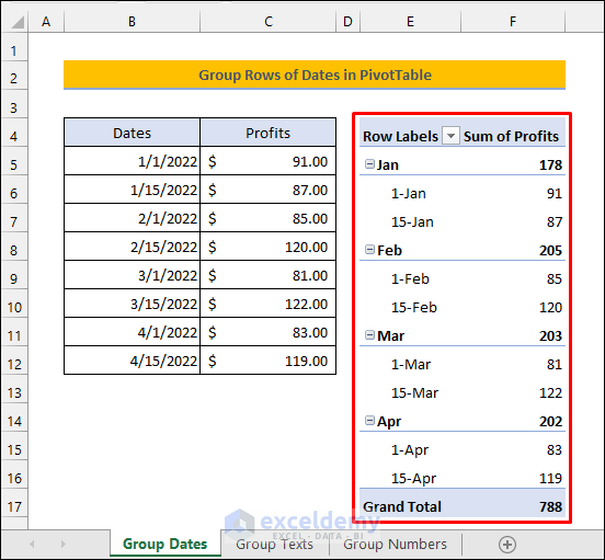
- After that, excel will automatically detect the starting and ending dates for grouping. You can change them as required. Then, select Days and Months to group By. Next, hit OK.

Finally, the rows of dates in the PivotTable will be grouped as follows.
Read More: How to Group Columns in Excel Pivot Table
2. Grouping Rows of Texts in Pivot Table
Now, assume you have the following Excel PivotTable instead. It contains a list of employee names and sales made by them.

- Now you can try to select a name and group them as in the earlier method. But, this time excel will through the following error.

- Therefore, you need to group the text values manually. First, select the texts that you want to group. Then, right-click and select Group as earlier.
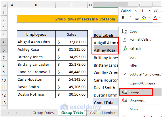
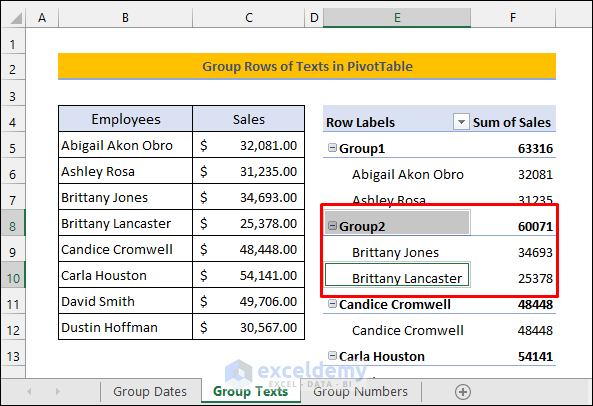
- After that, you will see them grouped together as follows.

- Try to do the same for the other texts. You can hold CTRL and then select to do that.

- Then, you will get a similar result.
- After, grouping all the texts, the PivotTable will look like the following one.
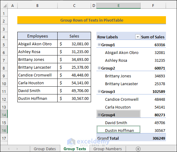
- Now, select a group and start typing to change its name. Then, press ENTER.

- Then, the PivotTable will be like the one below.

- You can use the hide buttons to hide the group contents. This way the PivotTable will look more concise.
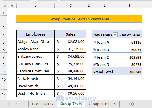
- You can also change the header names of the table.

Read More: How to Group Numbers in Excel Pivot Table
3. Grouping Rows of Numbers in Excel Pivot Table
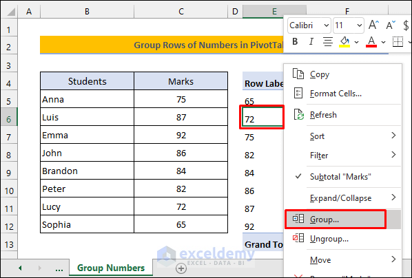
Now suppose that you have created an Excel PivotTable like the one shown below using a report card of some students.

- Now select any number in the Row Labels of the table. Then right-click and select Group as shown below.
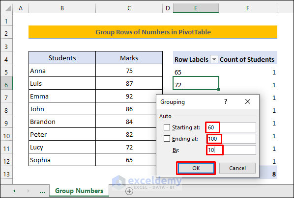
- Then, enter the Starting (60) and Ending (100) numbers and the difference (10) by which you want to group them. Next, hit OK.
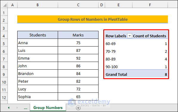
Finally, you will see the numbers grouped together as shown in the picture below.👇
Read More: How to Make Group by Same Interval in Excel Pivot Table
Things to Remember
- You can only group rows or columns in an Excel PivotTable.
- You will always need to manually select the rows of texts to group them.
Download Practice Workbook
You can download the practice workbook from the download button below.
Conclusion
Now you know how to group rows in the Excel Pivot Table. Please let us know if this article has helped you with the problem you were looking for. You can also use the comment section below for further queries or suggestions. Stay with us and keep learning.
Related Articles
- How to Use Excel Pivot Table to Group by Different Intervals
- Pivot Table Custom Grouping
- How to Rename a Default Group Name in Pivot Table
- [Fixed] Excel Pivot Table: Cannot Group That Selection
<< Go Back to Group Pivot Table | Pivot Table in Excel | Learn Excel
Get FREE Advanced Excel Exercises with Solutions!
