In this article, you’ll find a collection of the top 50 MCQs related to Excel formulas, along with their corresponding answers. These questions cover fundamental concepts and are suitable for both job-related assessments and academic examinations. If you have a basic understanding of Excel, you should be able to tackle these questions.
Before we dive into the MCQs, make sure you’re familiar with the following:
- Basics of an Excel spreadsheet
- Usage of the INDEX-MATCH formula
- Application of functions like AGGREGATE, AVERAGE, AVERAGEIF, CEILING.MATH, COUNT, COUNTBLANK, IF, IFS, COUNTIF, COUNTA, COUNTIFS, DATEDIF, DAY, FIND, IFERROR, LEN, MROUND, RAND, RANDBETWEEN, ROW, ROWS, SUM, SUMIF, TODAY, VLOOKUP, and XLOOKUP.
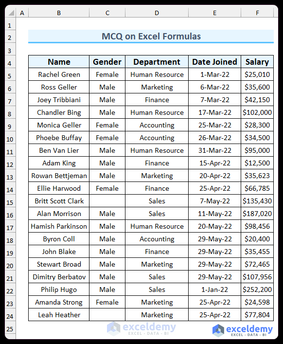
The questions are provided in the Problem sheet and the answers are highlighted in the Solution sheet. Below you can see a snapshot of the sample dataset for this article below. This dataset represents the data for twenty employees of a particular company.
Now, let’s go through the MCQ on Excel formulas.
- Q1. To find the number of empty cells, which formula would you use?
- (a) =COUNT(B5:F24)
- (b) =COUNTA(B5:F24)
- (c) =COUNTBLANK(B5:F24)
- (d) =DCOUNT(B5:F24)
- Q2. How can you display the applied formula for a cell?
- (a) =FORMULATEXT(Cell_Reference)
- (b) =TEXTFORMULA(Cell_Reference)
- (c) =FORMULASTEXT(Cell_Reference)
- (d) =SHOWFORMULA(Cell_Reference)
- Q3. Which of the following functions will you use to count the numbers in the dataset?
- (a) =COUNT(B5:F24)
- (b) =COUNTA(B5:F24)
- (c) =COUNTNUM(B5:F24)
- (d) =DCOUNT(B5:F24)
- Q4. To find the maximum salary, which formula(s) can you use?
- (a) =MAX(F5:F24)
- (b) =LARGE(F5:F24,1)
- (c) =AGGREGATE(4,0,F5:F24)
- (d) All of the above
- Q5. How do you calculate the mean of salaries?
- (a) =AGGREGATE(2,0,F5:F24)
- (b) =AVERAGE(F5:F24)
- (c) =MEAN(F5:F24)
- (d) All of the above
- Q6. Which formula returns 0?
- (a) =COUNTA(C5:C24)
- (b) =COUNT(C5:C24)
- (c) =COUNTBLANK(C5:C24)
- (d) None of these
- Q7. How many functions are included in the AGGREGATE function?
- (a) 17
- (b) 18
- (c) 19
- (d) 20
- Q8. To find the string size (number of characters) for the name column, which formula should you use?
- (a) =LEN(B5:B24)
- (b) =SIZE(B5:B24)
- (c) =STRINGLENGTH(B5:B24)
- (d) =LENGTH(B5:B24)
- Q9. To count the number of employees whose names begin with “R,” which formula is appropriate?
- (a) =COUNTIF(B5:B24,R*)
- (b) =COUNTIF(B5:B24,”R*”)
- (c) =COUNTIF(B5:B24,”R”)
- (d) =COUNTIF(B5:B24,”*R”)
- Q10. How can you calculate the space position in the name column?
- (a) =FIND(” “,B5:B24,1)
- (b) =SEARCH(” “,B5:B24,1)
- (c) =AGGREGATE(” “,B5:B25,1)
- (d) Both a & b
- Q11. What’s the difference between the SEARCH and FIND functions?
- (a) The FIND function is case sensitive, and the SEARCH function is not.
- (b) The SEARCH function is case sensitive, and the FIND function is not.
- (c) There is no difference between them, only for compatibility, both are listed.
- (d) None of these.
- Q12. Which function can be used to find the number of females?
- (a) COUNTIFS
- (b) COUNTIF
- (c) COUNT
- (d) Both a & b
- Q13. Which function finds the highest salary value?
- (a) MAX
- (b) MAXIMUM
- (c) AGGREGATE
- (d) Both a & c
- Q14. How can you calculate the total value of salaries for male employees?
- (a) SUMIF
- (b) IFS
- (c) MAX
- (d) INDEX-MATCH
- Q15. To find the employee who received the highest salary, which formula should you use?
- (a) =INDEX(B5:B24,MATCH(MAX(F5:F24),F5:F24,0))
- (b) =INDEX(B5:B24,MATCH(MAX(F5:F24),F5:F24,1))
- (c) =INDEX(B5:B24,MAX(F5:F24),0)
- (d) =INDEX(B5:B24,MATCH(MAX(F5:F24),F5:F24,-1))
- Q16. How can you find distinct job department names?
- (a) AGGREGATE
- (b) UNIQUE
- (c) Combination of IFERROR, INDEX, MATCH
- (d) Both b & c
- Q17. Which feature(s) can be used to extract the day value from the “Date Joined” column?
- (a) DAY Function
- (b) Insert an adjacent helper column and use Flash Fill
- (c) LEFT Function
- (d) Both a, b & c
- Q18. Which function determines the number of empty cells in the dataset?
- (a) COUNT
- (b) COUNTA
- (c) COUNTBLANT
- (d) COUNTBLANK
- Q19. Which function returns a random name from the list?
- (a) =INDEX(B5:B24,MATCH(RANDBETWEEN(1,20),B5:B24,0))
- (b) =INDEX(B5:B24,RANDBETWEEN(1,20))
- (c) =INDEX(B6:B25,RAND())
- (d) =INDEX(B6:B25,RAND(20))
- Q20. To determine the number of salaries greater than $100,000 AND dates joined after 30th April, which formula should you use?
- (a) =COUNTIFS(F5:F24,”>100000″,E5:E24,”>44681″)
- (b) =COUNTIF(F5:F24,”>100000″)+COUNTIF(E5:E24,”>44681″)
- (c) Both a & b
- (d) None of these
- Q21. To determine the number of salaries greater than $100,000 OR dates joined after 30th April, which formula should you use?
- (a) =COUNTIFS(F5:F24,”>100000″,E5:E24,”>44681″)
- (b) =COUNTIF(F5:F24,”>100000″)+COUNTIF(E5:E24,”>44681″)
- (c) Both a & b
- (d) None of these
- Q22. How can you calculate the average salary for male employees?
- (a) =AVERAGEIF(C5:C24,”Male”,F5:F24)
- (b) =AVERAGEIFS(C5:C24,”Male”,F5:F24)
- (c) =IF(C5:C24=”Male”,AVERAGE(F5:F24),””)
- (d) =MEANIF(C5:C24,”Male”,F5:F24)
- Q23. Which function calculates the arithmetic mean?
- (a) MEAN
- (b) AVERAGE
- (c) GEOMEAN
- (d) MIDPOINT
- Q24. What shortcut applies the SUM function?
- (a) Alt+=
- (b) Ctrl+=
- (c) Shift+=
- (d) Ctrl+Alt+=
- Q25. To retrieve a value from the left side of a matched value, which function can you use?
- (a) VLOOKUP Function
- (b) Combination of VLOOKUP and IF Functions
- (c) HLOOKUP Function
- (d) ZLOOKUP Function
- Q26. Which formula correctly returns the name of the employee with a salary of $25,010?
- (a) =VLOOKUP(F5,IF({1,0},F5:F24,B5:B24),2,0)
- (b) =ZLOOKUP(F5,F5:F24,B5:B24)
- (c) =XLOOKUP(F6,F5:F24,B5:B24)
- (d) Both a&c
- Q27. If cell C15 is empty and F15 contains $135,430, what is the result of C15*F15?
- (a) $135,430
- (b) 0
- (c) #VALUE!
- (d) #DIV/0
- Q28. Which function determines the number of values in the Salary column?
- (a) NUM
- (b) NUMBER
- (c) COUNT
- (d) None of these
- Q29. To display the current date along with the time, which function(s) can you use?
- (a) =NOW()
- (b) =TODAY()
- (c) Both
- (d) None of these
- Q30. Which formula rounds up the salary figure from cell F17 to the nearest thousand?
- (a) =MROUND(F17,1000)
- (b) =FLOOR.MATH(F17,1000)
- (c) =CEILING.MATH(F17,1000)
- (d) =ROUNDUP(F17,1000)
- Q31. How can you assign sequential serial numbers (1, 2, 3, etc.) to the rows using a formula and AutoFill?
- (a) =ROWS($B$5:B5)
- (b) =ROWS(B5)
- (c) =ROW(B5)-3
- (d) Both a&c
- Q32. Which of the following are not valid Excel functions?
- (a) NUM
- (b) MEANS
- (c) TRUE
- (d) Both a&b
- Q33. Which function is available but not shown in Excel Tooltip?
- (a) DATEVALUE
- (b) DATEDIF
- (c) KLOOKUP
- (d) DCOUNT
- Q34. To fix a cell reference, which symbol do you use?
- (a) $
- (b) !
- (c) *
- (d) %
- Q35. What is the Not Equal operator in Excel?
- (a) =!
- (b) <>
- (c) !=
- (d) ||
- Q36. What is a circular reference in an Excel formula?
- (a) A reference that relies on itself
- (b) A type of the absolute cell reference
- (c) A reference that Speeds up calculation
- (d) None of these
- Q37. Which shortcut fills down a formula?
- (a) Ctrl+D
- (b) Alt+D
- (c) Shift+D
- (d) Ctrl+Alt+D
- Q38. Which shortcut is used to activate the Flash Fill feature?
- (a) Ctrl+F
- (b) Ctrl+E
- (c) Alt+E
- (d) Alt+F
- Q39. To display the remainder after dividing 100 by 3, which function should you use?
- (a) =MOD(100,3)
- (b) =DIV(3,100)
- (c) =MODE(100,3)
- (d) =REMAINDER(100,3)
- Q40. How do you concatenate values in a formula?
- (a) Semicolon (;)
- (b) Comma (,)
- (c) Ampersand (&)
- (d) Pipe (|)
- Q41. Which is the latest lookup function?
- (a) KLOOKUP
- (b) XLOOKUP
- (c) VLOOKUP
- (d) LOOKUP
- Q42. A formula must begin with:
- (a) =
- (b) +
- (c) –
- (d) (
- Q43. Which of the following formulas contains an error?
- (a) =F7+F8
- (b) =F9+F11
- (c) (F9+F11)
- (d) No error
- Q44. o find the output of a formula, you need to select the full formula or a portion of it and press X to show the output. What does X represent?
- (a) F7
- (b) F8
- (c) F9
- (d) F10
- Q45. How can you refer to a cell reference from another worksheet?
- (a) navigate to the sheet and click on that cell
- (b) type the sheet name, add !, and include the cell address
- (c) both of these
- (d) It is not possible in Excel
- Q46. Which of the following functions was introduced in Excel 2019?
- (a) UNIQUE
- (b) IFS
- (c) FLOOR.MATH
- (d) XLOOKUP
- Q47. Which function can handle all kinds of errors?
- (a) IFNA
- (b) IFERROR
- (c) ISERROR
- (d) ALLERROR
- Q48. How can you insert formulas?
- (a) Typing the formula
- (b) Using Insert Function feature from the Functions tab
- (c) Any of the above two
- (d) None of these
- Q49. Which function removes extra spaces?
- (a) TRIM
- (b) TRUNC
- (c) CODE
- (d) DELETE
- Q50. Which of the following functions is a Statistical function?
- (a) GESTEP
- (b) DEVSQ
- (c) BITXOR
- (d) IMSUB
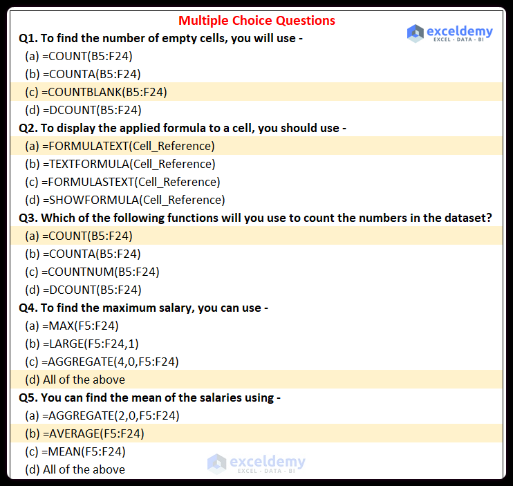
The image below depicts the first five solutions to the MCQ on Excel formulas. The solutions to the questions have been highlighted.
Download Practice Workbook
You can download the Excel file from the following link.

