Method 1 – Make Generic Time Attendance Sheet
Step 1: Assign Date & Day
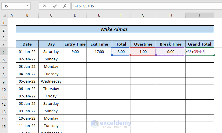
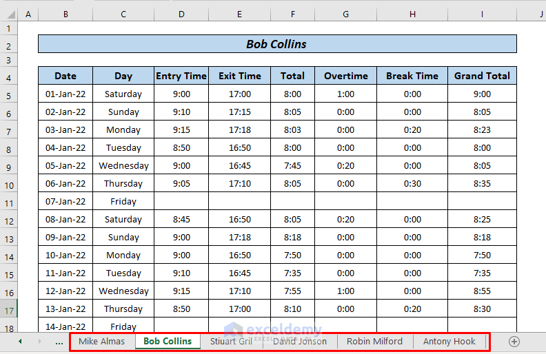
- Create a sheet table for one of the employees (i.e. Mike Almas) with multiple headings (i.e. Date, Day, Entry Time, Exit Time, Over Time, Break Time, etc.). Assign the date range and day for this sheet table. (we used it just for 1 month. Proceed with your acquainted time period).
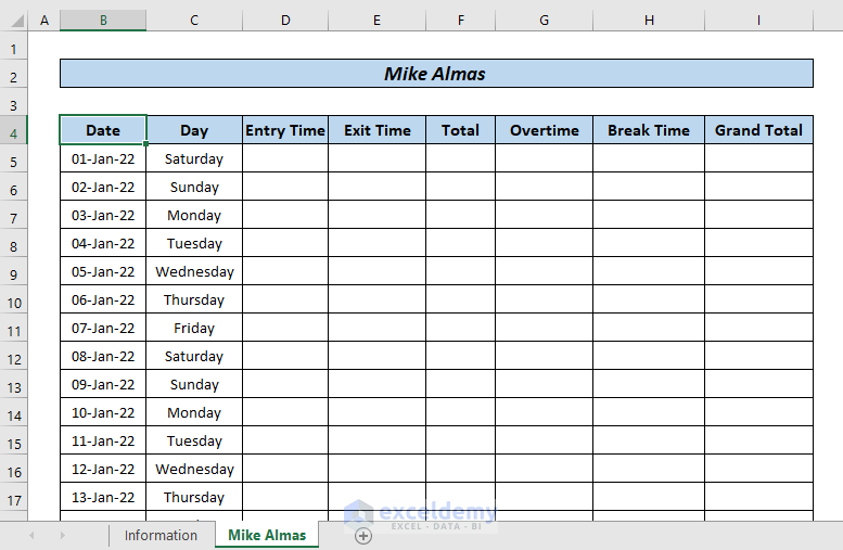
- Select the row just below the header row> go to the View tab> click Freeze Panes> select Freeze Panes.
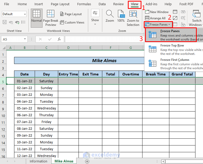
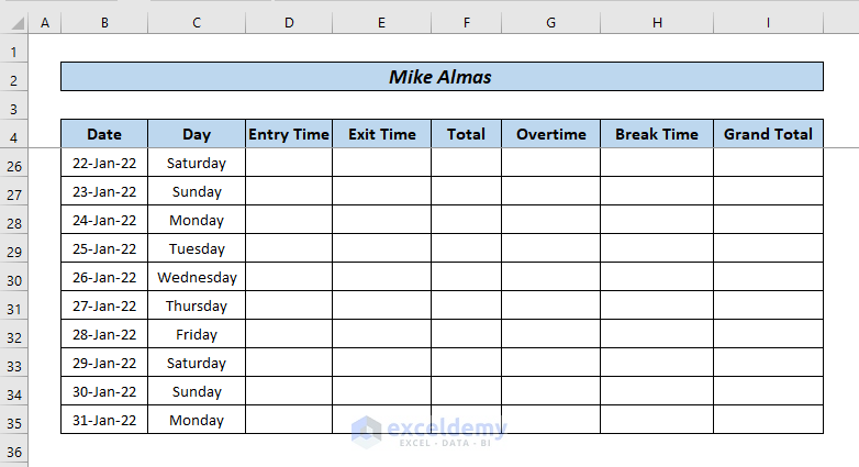
- Freezing panes will allow the header row not to move anymore with scrolling down the cursor.
Step 2 – Assign Entry & Exit Time and Get Attendance
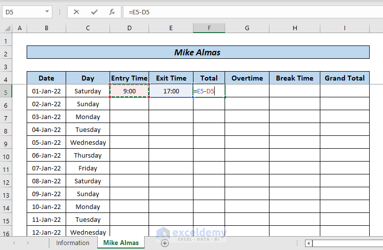
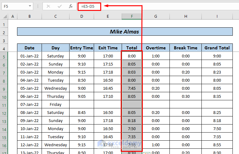
- Enter the Entry Time and Exit Time to the respective cell and apply the following formula to the cell where you want to show the working hour from entry to exit:
=E5-D5
- E5= Entry Time
- D5= Exit Time
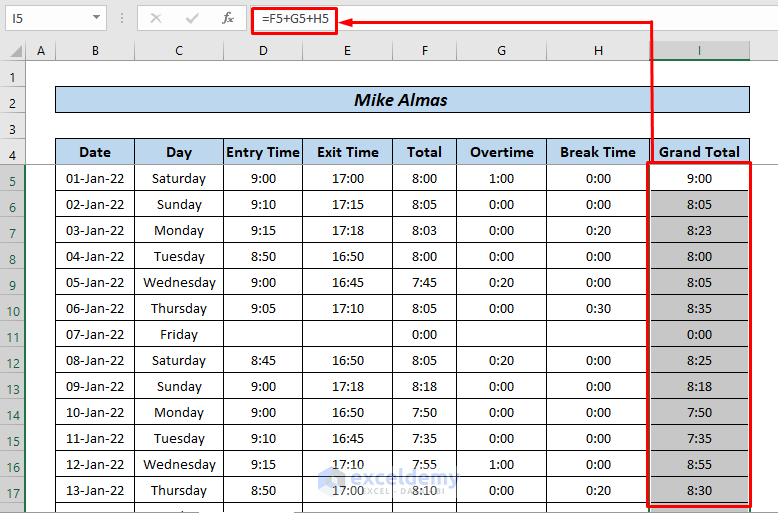
- Assign the Overtime and Break Time and apply the following formula for getting the grand total of the working hours:
=F5+G5+H5
- F5= Total (between Entry and Exit)
- G5= Overtime
- H5= Break Time
- Hit ENTER to get the output.
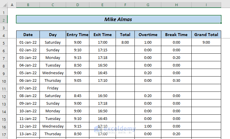
- Enter the respective time every day and use the Fill Handle Tool to drag the formula down the cells to get the corresponding result.
- Grand Total denotes the total working hours, including overtime and break time.
Step 3 – Holidays in Attendance Sheet
- The holidays (i.e., Friday), the value in the Total and the Grand Total cell will also exist. Removing them will remove the formula so avoid it. Rather select the cells for holidays> go to the Home tab> click Font Color> choose the font color just like the fill color of the cell (i.e. White).
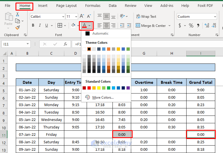
- Your cell won’t show the cell value. They exist, but they won’t show up because of the fill color.
- Create extra sheets for the other employees and repeat this same procedure for everyone.
Method 2 – Create Attendance Sheet with Presence and Absence
Step 1: Create Month Name
- Select a cell and add the following formula:
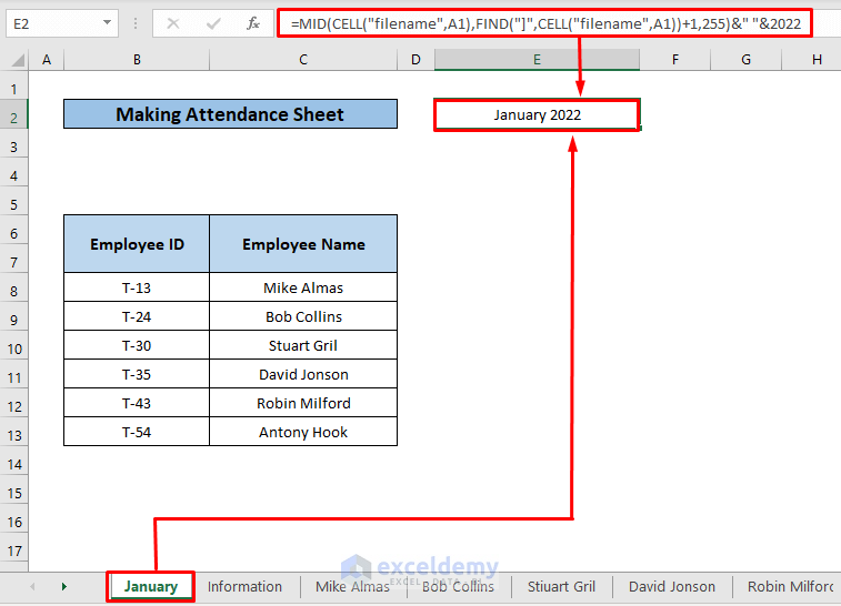
=MID(CELL("filename", A1), FIND("]", CELL("filename", A1))+1,255)&" "&2022
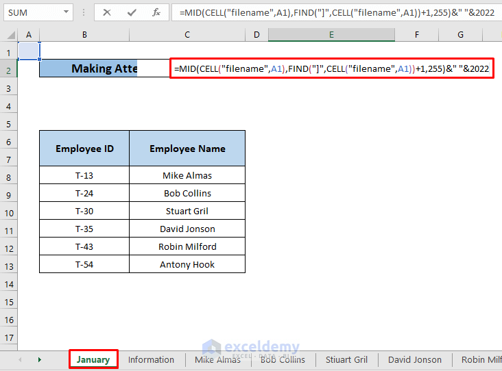
- Hit ENTER and the cell will return the value. Set the sheet name as January as we want to make a sheet for this month.
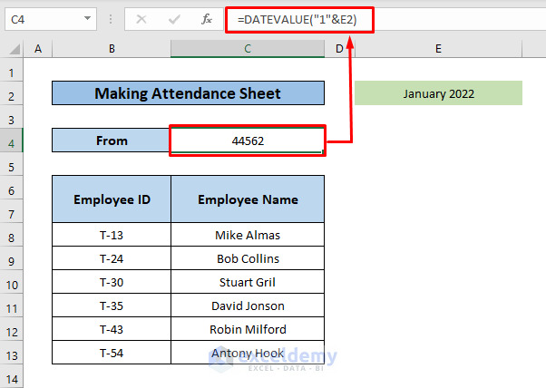
- Select a cell for the start date of the month and apply the DATEVALUE function:
=DATEVALUE(“1”&E2)
- E2= Month of January
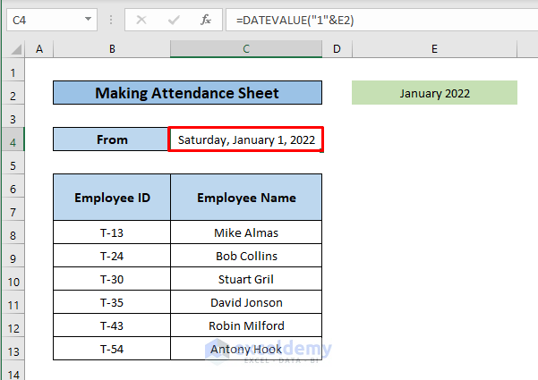
- Go to the Home tab> Number Format> select Long Date.
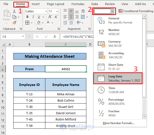
- The cell will show the long date format.
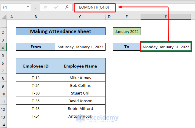
- Select another cell for the end date and apply the formula below:
=EOMONTH(C4,0)
- C4= Start Date
Step 2: Assign Respective Date & Day
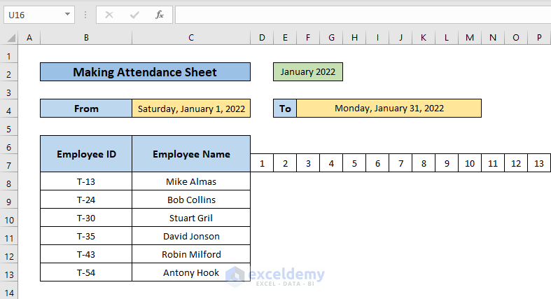
- Choose a cell where you want to put the first date of the month and apply:
=C4
- C4= Start Date of the Month
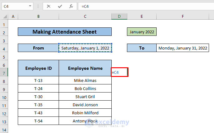
- Hit ENTER.
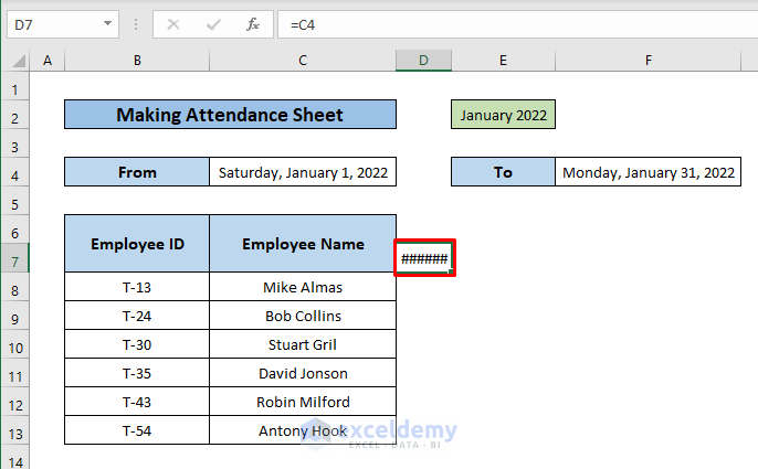
- Click CTRL+1 to open the Format Cells dialogue box. From the Custom icon, select d from Type> click OK.
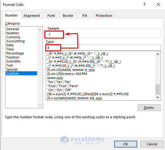
- The cell will show 1. (as date)
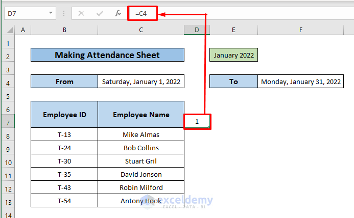
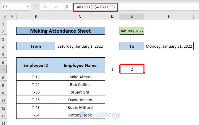
- Apply the IF function and assign the following formula to the next cell:
=IF(D7<$F$4,D7+1,"")
- D7= 1 (first date)
- Use the Fill Handle tool to drag the formula to the right cells to till it completes the day of the month.
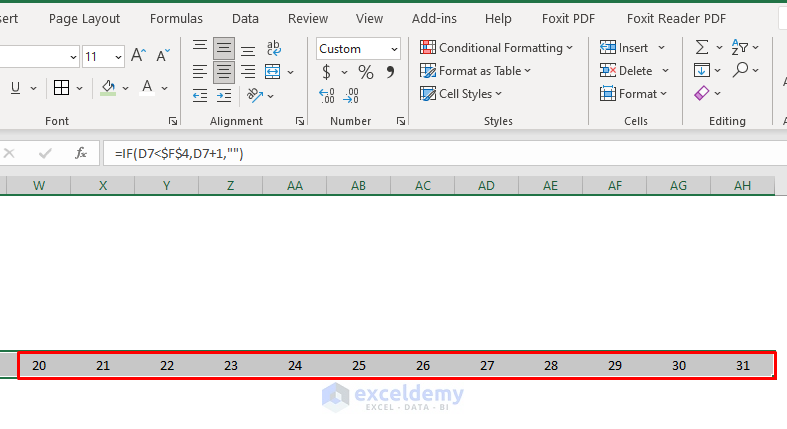
- The cells will show the dates.
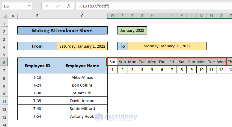
- Apply the TEXT function and assign the following formula to the upper cell to get the day:
=TEXT(D7,”ddd”)
- D7= date
- ddd= first e letters of the day
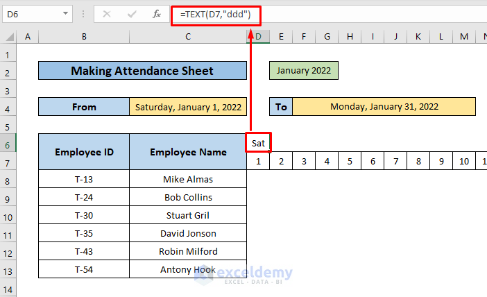
- Drag the formula to the right end.
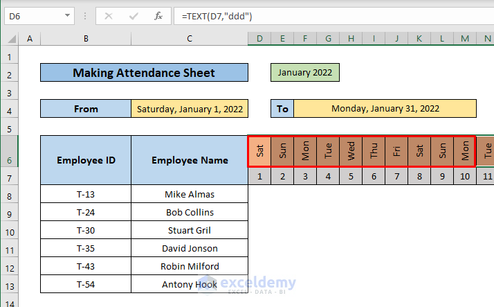
- Select all the days>click CTRL+1 and from the Format Cells dialogue box, select Alignment> type 90 in the degree section> click OK.
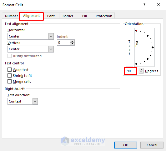
- The days will be aligned to 90 degrees.
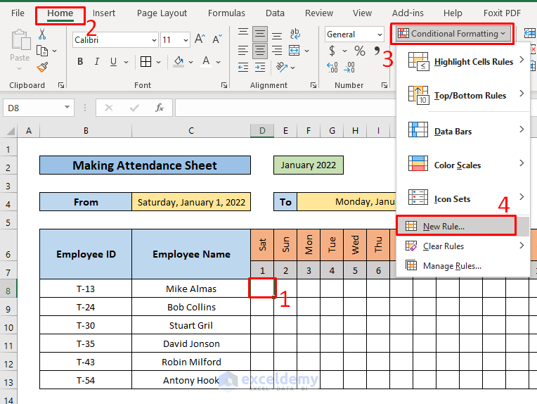
Step 3: Apply Conditional Formatting
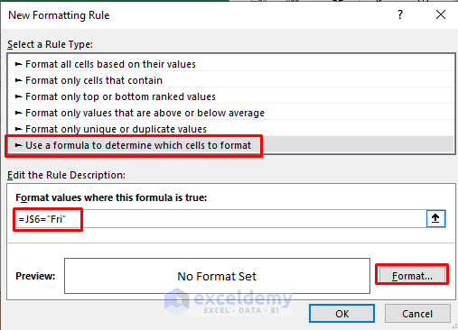
- Select the cell for the first day of the first employee> go to the Home tab> Conditional Formatting> New Rule.
- Select the last rule from the list>write the formula> click Format:
=J$6=”Fri”
- Fri= Holiday (as we want to format cells for holiday)
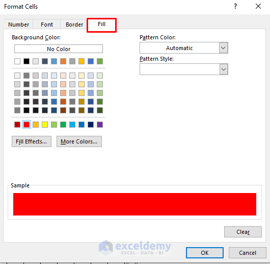
- Select a fill color> click OK.
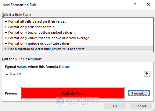
- Click OK on the New Formatting Rule box.
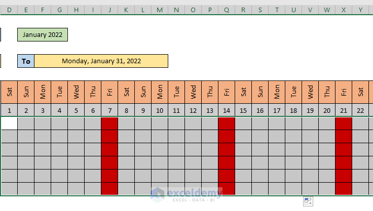
- Drag the formula to the last date and last person and the cells for holidays will be formatted as red like below.
Step 4: Assign Attendance as Present and Absent
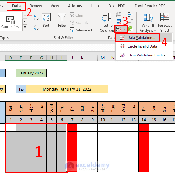
- Select the blank cells (i.e. the working dates)> go to Data tab> Data Validation.
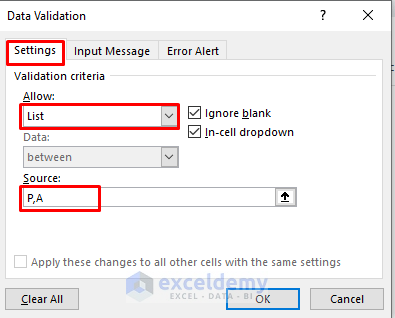
- The Data Validation box will appear. Select List from Allow and assign P, A (denoting Present/ Absent) to Source box>click OK.
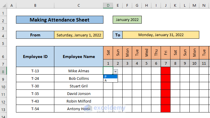
- The drop-down button will appear for the selected cells. You can choose P or A from here to denote the Presence or Absence of an employee.
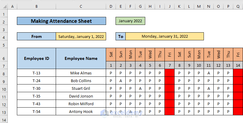
- Assign the attendance for the sheet table.
- Select the attendance> go to Home tab> Conditional Formatting> Highlight Cells Rules> Text that Contains.
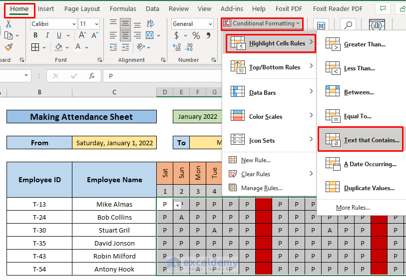
- Choose a fill for P> click OK.
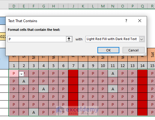
- P will be formatted, and you can easily distinguish between presence and absence.
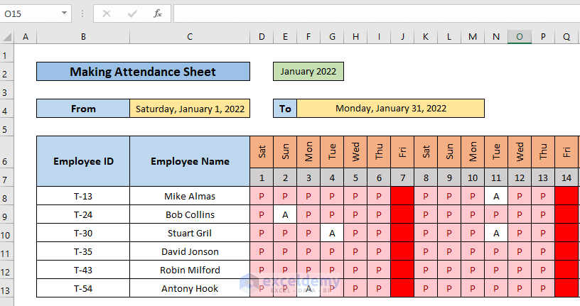
You can make an attendance sheet with presence and absence in Excel.
Download Practice Workbook
<< Go Back to Formula List | Learn Excel
Get FREE Advanced Excel Exercises with Solutions!
