The sample workbook will provide a few different scenarios for when you need to calculate YTD in Excel, such as YTD price, profit, or growth rate.
Method 1 – Calculating YTD with SUM Functions
Consider a business company that has sold a number of products in 12 months of a year, with the total selling prices for all months recorded in the sample table. To learn the Year-to-Date selling price per unit quality of the products for each month, use the SUM function by following these steps.
Steps:
- Type the formula in cell E5.
=SUM($D$5:D5)/SUM($C$5:C5)- Press Enter to find the YTD for the first month.
- Use the Fill Handle to AutoFill the formula to the whole column.
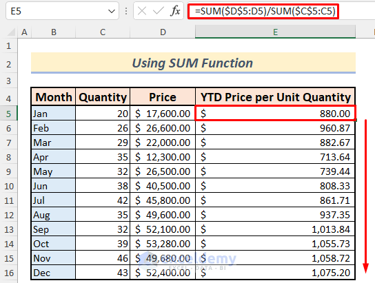
The formula here is working through the division between two cumulative values for price and quantity. Here the divided part is cumulative prices for the products, and the divisor part is cumulative sums of the quantity of the products.
Read More: How to Sum Year to Date Based on Month in Excel
Method 2 – Applying Excel Combined Functions to Calculate YTD
You can also calculate the YTD Price Per Unit using the combination of SUM, IF, MONTH, and OFFSET functions.
Steps:
- Make some modifications in the Month column to include a specific date. Say you’re taking accounts on the 28th day of each month. So, the first date will be 1/28/2021.
- Type the following formula in cell E5 and press the ENTER button. You will see the YTD Price Per Unit in January.
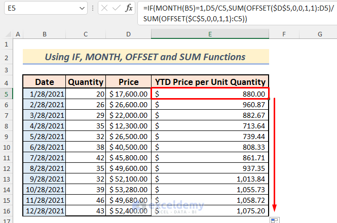
=IF(MONTH(B5)=1,D5/C5,SUM(OFFSET($D$5,0,0,1,1):D5)/SUM(OFFSET($C$5,0,0,1,1):C5))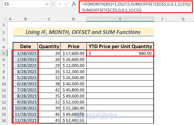
The formula references cells D5 and C5 using the OFFSET function. It removes the Formula Omits Adjacent Cells error. The IF function returns the Price per Unit of January if the month in B5 is the first month of the year. Otherwise, it returns values for the later months of the year.
- Use the Fill Handle to AutoFill the lower cells.
Method 3 – Calculating YTD Using Excel SUMPRODUCT Functions
Steps:
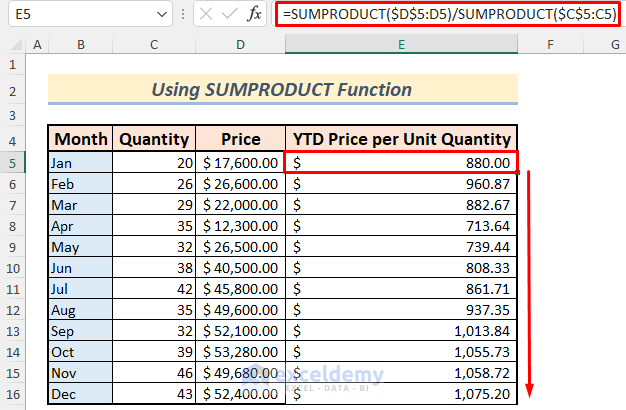
- Type the following formula in cell E5:
=SUMPRODUCT($D$5:D5)/SUMPRODUCT($C$5:C5)- Press Enter to receive the result for the first month.
- Use the Fill Handle to autofill the whole column.
Method 4 – Determining YTD Growth Rate by Using a Dynamic Formula
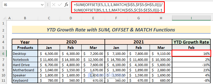
Let’s compare sales data between two years for fixed successive months with YTD (see example table below). Specifically, the example will determine the YTD for the months of January & February to compare sales data between two years- 2020 & 2021. The useful functions for this method are SUM, OFFSET, and MATCH functions.
Steps:
- Type the following formula on cell I6:
=SUM(OFFSET(E5,1,1,1,MATCH($I$5,$F$5:$H$5,0)))/SUM(OFFSET(B5,1,1,1,MATCH($I$5,$C$5:$E$5,0)))-1- Press Enter.
- Under the Home ribbon, select Percentage from the drop-down in the Number group of commands. The decimal value will be turned into a percentage.
- Use the Fill Handle to AutoFill other YTD growth rates for all products.
Method 5 – Calculating YTD Profits by Incorporating Excel Functions
You can find YTD values up to a particular month by inserting a specific date by using SUM, OFFSET, ROWS, and MONTH functions.
Steps:
- Go to cell I7 and insert the following:
=SUM(OFFSET($C$6,ROWS($B$7:B7),0,,MONTH($C$4)))- Press Enter.
- Autofill other cells in column I for all other products by using the Fill Handle.
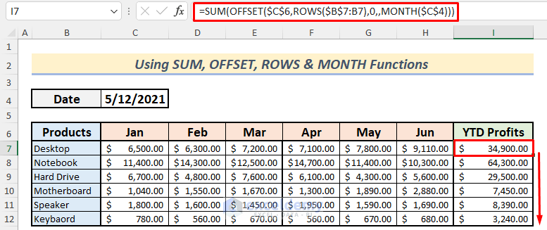
For the example, the input date is May 12, 2021. The MONTH function extracts the month from this date, which formula then uses as the column number up to which the calculation will be executed.
Read More: How to Calculate MTD (Month to Date) in Excel
Method 6 – Calculating YTD by Using Excel SUMIFS Functions
You can extract year, month, and date values with the help of YEARFRAC and DATE functions, and then use them to find the YTD rate. For the sample dataset, selling prices of the products for 10 days have been recorded along with their cost prices. To determine the YTD profit rates for successive 10 days using the SUMIFS function, read below.
Steps:
- First, type the following formula in cell F5.
=YEARFRAC(DATE(E5,1,1),B5,1)- Press Enter. This results in the fraction or percentage of the days up to the particular date in column B based on 365 days in a year.
- Use the Fill Handle to fill down the whole column F.
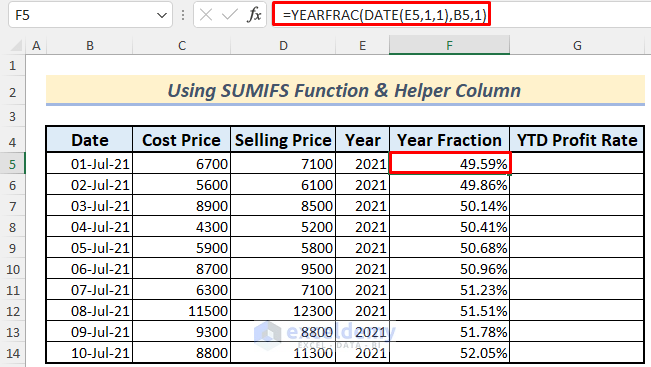
The YEARFRAC function returns the year fraction representing the number of whole days between start_date and end_date. The DATE function inside inputs the first day of the year 2021 (listed in E5).
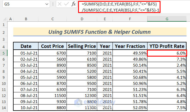
- Go to cell G5 and type the formula below.
=SUMIFS(D:D,E:E,YEAR(B5),F:F,"<="&F5)/SUMIFS(C:C,E:E,YEAR(B5),F:F,"<="&F5)-1- Press Enter.
- Go to the Home tab, Number group, and select the percentage icon (%).
- Fill down the whole column G to get the YTD profit rates for all successive 10 days at once.
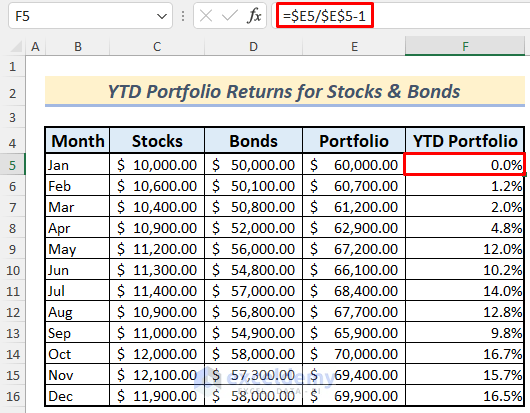
Method 5 – Determining YTD Portfolio Returns for Stocks & Bonds
Steps:
- In cell F5, write down this formula:
=$E5/$E$5-1- Press Enter to get the first value as 0.
- Convert the whole column into a percentage by selecting the percentage icon in the Number section.
- Drag the Fill Handle to AutoFill the other YTD returns for all months.
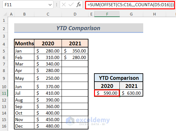
Method 8 – Merging Excel Functions Together to Compare YTD
To compare the cumulative values between two specific and successive timespans from two different years, you’ll need to combine a few functions. Here, the sales values for all months in 2020 are presented in column C. When you input a value in column D you’ll get the comparative results up to that specific month between the two years. This uses SUM, OFFSET, and COUNTA functions.
Steps:
- Type the following formula in cell F11:
=SUM(OFFSET(C5:C16,,,COUNTA(D5:D16)))- Press Enter and you’re done with the YTD for the year 2020.
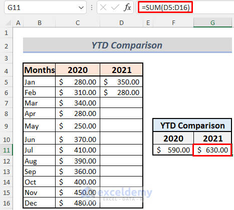
- Put the following formula in cell G11.
=SUM(D5:D16)- Press Enter to finish.
When you input data in column D, cells F11 as well as G11 will simultaneously show YTD values up to the specific months for the years 2020 and 2021 respectively. This is due to the formula in F11 working through year 2020, but only up to the months filled in 2021.
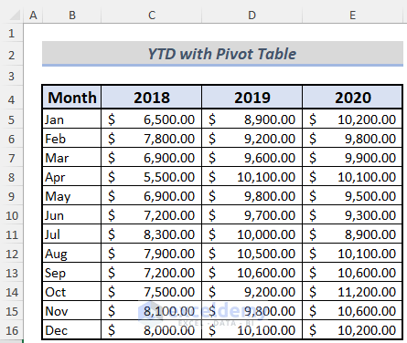
Method 9 – Creating Pivot Table to Calculate YTD
Consider a table for the sales values of three successive years.
Steps:
- First, select the whole table and choose the Pivot Table option from the Insert ribbon.
- Put Months in the Rows Field and the Year headers in the Values Field.
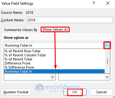
- Put your mouse cursor on any of the sales values in the year 2018 and open Value Field Settings from the options by right-clicking.
- Select the Show Values As tab and Running Total In.
- Press OK to get the cumulative sales value or running total for the year of 2018.
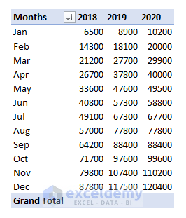
- Repeat this process for the years 2019 and 2020.
- You can see the output that shows YTD for all months for the three years.
How to Calculate YTD Average in Excel
Use the AVERAGE function to calculate the YTD average.
Steps:
- Type the following formula in cell D5.
=AVERAGE($C$5:C5)- Press Enter.
- Drag the Fill Icon to AutoFill the lower cells.
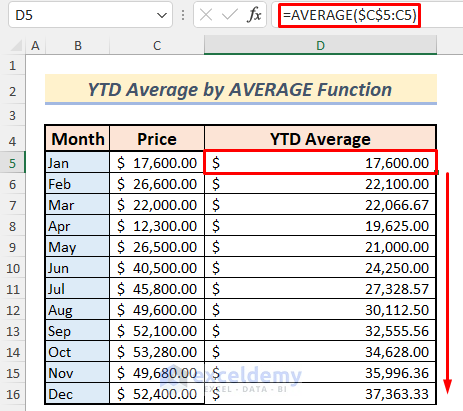
This calculate the YTD average per month.
Download Practice Workbook
You can download the Practice Workbook that we’ve used to prepare this article.
<< Go Back to Excel Formulas for Finance|Excel for Finance|Learn Excel
Get FREE Advanced Excel Exercises with Solutions!

I still have a question
When you want to see in a pivot table e.g YTD3 but for one line there are no entries in period 3 the pivot table shows for this period till YTD 2 how can I create a total into the zero entries to come to YTD3
Thank you for your inquiry, INGE. It is not really clear from your inquiry what you want. I believe you want to know how we can calculate the running total when a month’s entry is zero. In that situation, the Pivot table will add 0 to the previous running total, displaying the same prior running total as before. I hope this clarifies your concerns. If you have any further queries or wish to share your documents, please post them on our Exceldemy Forum (https://exceldemy.com/forum/).
Regards
Aniruddah