Method 1 – Calculating the Year-to-Date Sum Based on Monthly Input
Example Model:
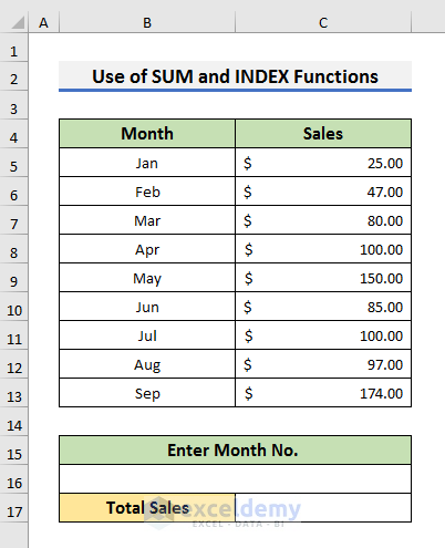
STEPS:
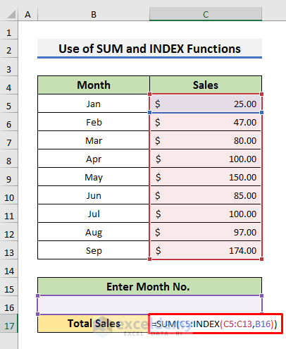
- Enter the following formula into cell C16.
=SUM(C5:INDEX(C5:C13,B16))Note: This formula will calculate the range from cell C5 {the starting month} to the given month.
- Insert the month and Press
- The result will be shown in C17.
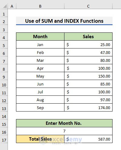
Note: no month can be used, only index values.
Read More: How to Calculate YTD (Year-To-Date) Average in Excel
Method 2 – Calculating the YTD Sum Using Dynamic Range
Example Model:
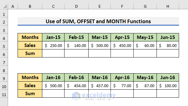
STEPS:
- Enter the following formula into cell B5.
=SUM(OFFSET(C5,0,0,1,-MONTH(C4)):C5)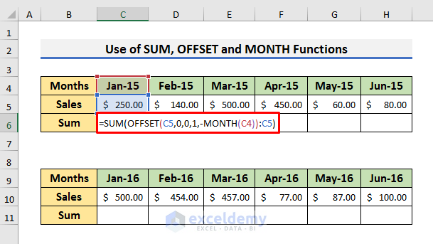
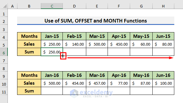
- Drag and fill the formula to the right in order to see the output.
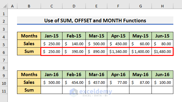
Results:
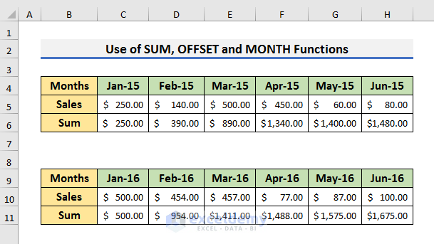
- Use the same formula for the other years in order to see the result.
Read More: How to Calculate YTD (Year-to-Date) in Excel
Method 3 – Calculating Sum Values Based on Month in Excel
Example Model:
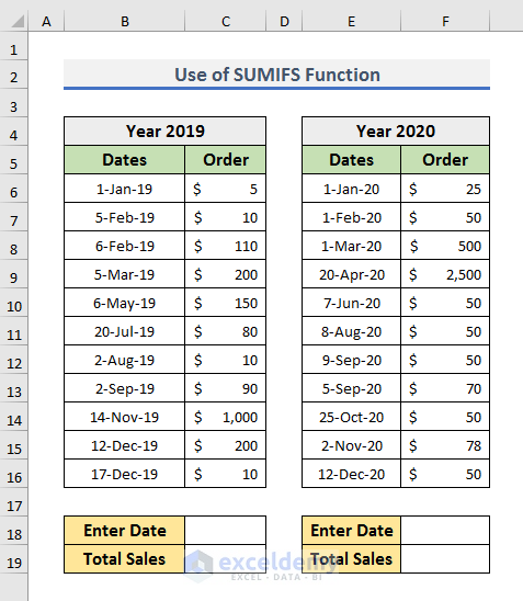
STEPS:
- Enter the following formula into cell C19.
=SUMIFS(C6:C16, B6:B16, ">="&B6, B6:B16, "<="&C18)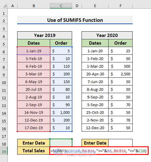
- Type any date into the input box (cell C18) and press Enter.
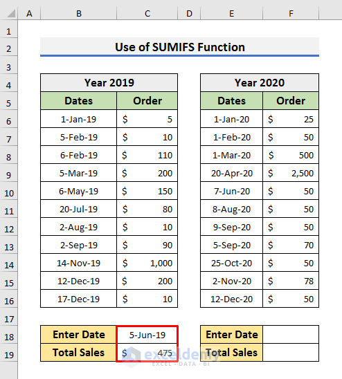
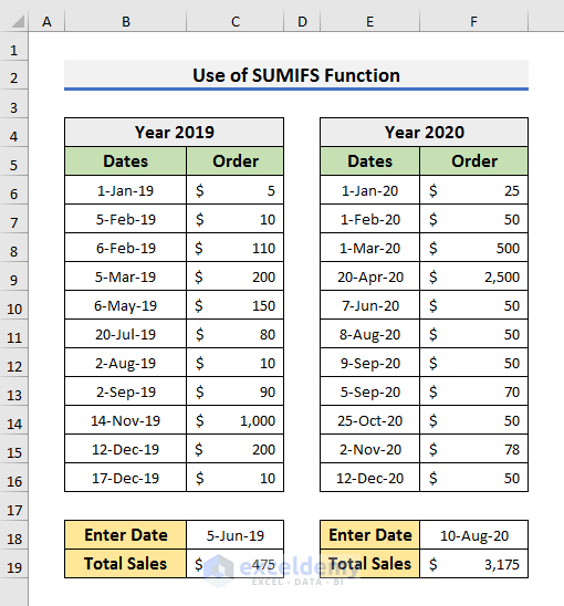
Note: You can check the other table’s formula by entering the date for the year 2020.
Method 4 – Calculate the YTD Sum with Excel IF Function
Example Model:
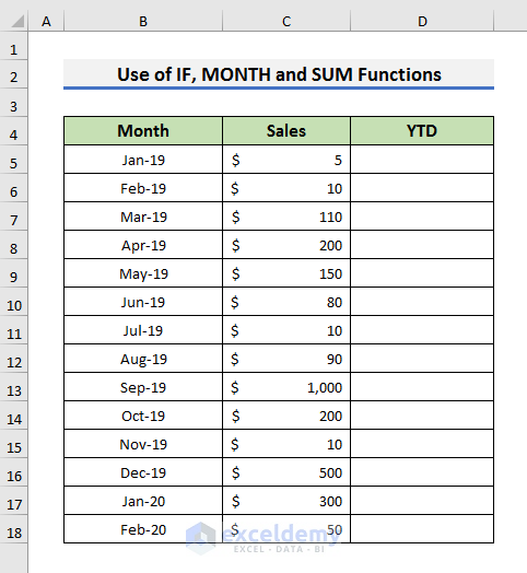
STEPS:
- Enter the following formula into cell D5.
=IF(MONTH(B5)=1,C5,SUM(C5,D4))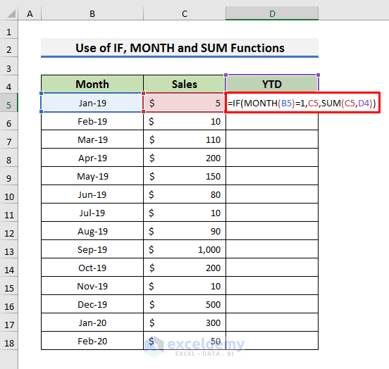
Note: The following formula
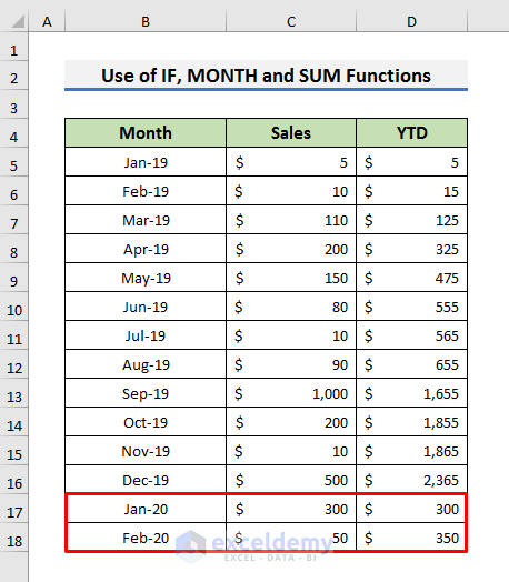
- Press Enter and drag the Fill Handle (+) down to cell D18.
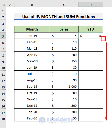
Note: D17 shows the year-to-date sum, it starts calculating the sum for the year 2020.
Download Practice Workbook
You can download the practice workbook from here.
Related Article
<< Go Back to Excel Formulas for Finance|Excel for Finance|Learn Excel
Get FREE Advanced Excel Exercises with Solutions!

I need a similar formula but for AVERAGE instead of SUM as the number of months keep growing. Can you help with that?
Hi KATIA,
Thanks for your comment. I am replying to you on behalf of Exceldemy. To find the average, you can use the AVERAGE function. For Method 1, you can follow the steps below.
STEPS:
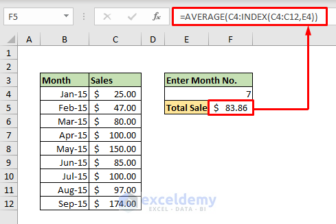
1. Firstly, select Cell F5 and type the formula below:
=AVERAGE(C4:INDEX(C4:C12,E4))2. Press Enter to see the result.
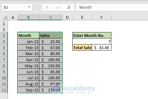
3. Secondly, select the range B3:C12.
4. Press Ctrl + T to convert the range into a table.
5. A message box will appear.
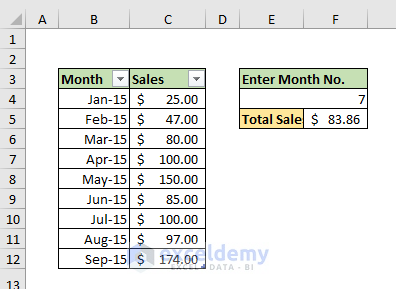
6. Click OK to proceed.
7. As a result, you will see a table like the picture below.
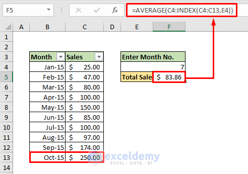
8. Now, if you add Oct-15 in Cell B13, then the table and formula of Cell F5 will automatically update.
For Method 2, you can follow the above steps and use the formula below:
=AVERAGE(OFFSET(B4,0,0,1,-MONTH(B3)):B4)For Method 3, use the formula below and convert the range into a table:
=AVERAGEIFS(C4:C17, B4:B17, ">="&B4, B4:B17, "<="&F5)You can also find the formulas in the workbook below:
Workbook with AVERAGE Formulas.xlsx
I hope this will help you to solve your problems. Please let us know if you have other queries.
Thanks!