How to Calculate MTD (Month to Date) in Excel (3 Methods)

Method 1 – Combine SUM, OFFSET, ROWS & DAY Functions to Calculate MTD in Excel

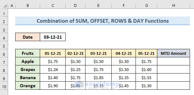
Suppose we have the following dataset of a fruit stall. The dataset contains the sales amount of different fruits for the first five days of the month. Now, we want to know the Month to Date amount for each fruit.

Steps:

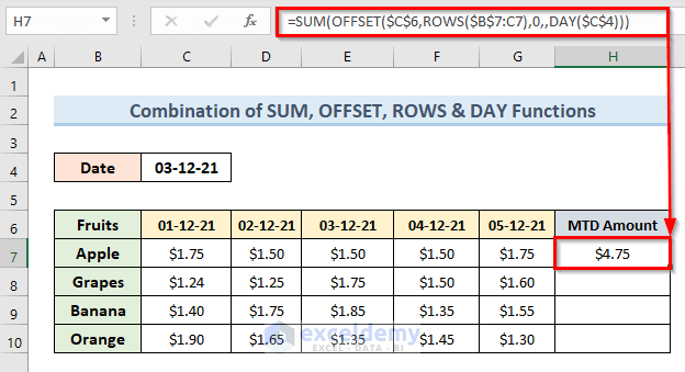
Select cell H7 and type the following formula:

=SUM(OFFSET($C$6,ROWS($B$7:C7),0,,DAY($C$4)))

Press Enter.
In cell H7, we will get the total sales value up to the date 3-12-21.

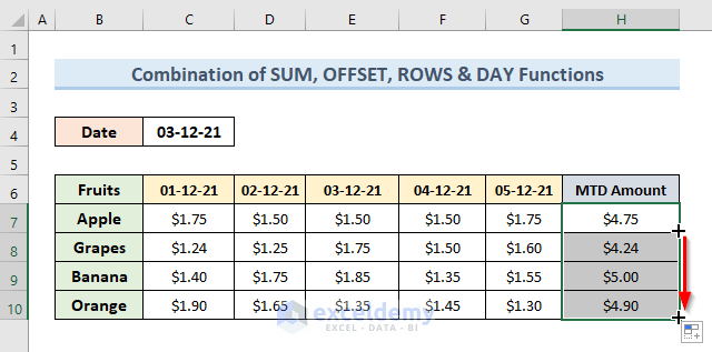
Drag the Fill Handle tool from cell H7 to H10 to get results for other fruits.

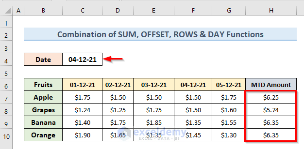
Change the date to 4-12-21 from 3-12-21. The MTD amount changes automatically.

How Does the Formula Work?

OFFSET($C$6,ROWS($B$7:C7),0,,DAY($C$4)): This part returns the range. The range is specified for row 7 taking cell C6 and the date of cell C4 as references.
SUM(OFFSET($C$6,ROWS($B$7:C7),0,,DAY($C$4))): This part returns the sum of sales amount up to the date in cell C4.

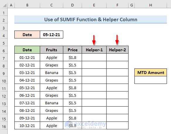
Method 2 – Calculate MTD in Excel with SUMIF Function & Helper Column

In the following dataset, we have sales data for a fruit stall. It gives us the sales amount for the first 10 days for different fruits.

Steps:

Insert two helper columns with the dataset.

Insert the following formula in cell E7.

=IF(B7<$C$4,MONTH($C$4),0)

Press Enter. The above formula returns 12 in cell E7.

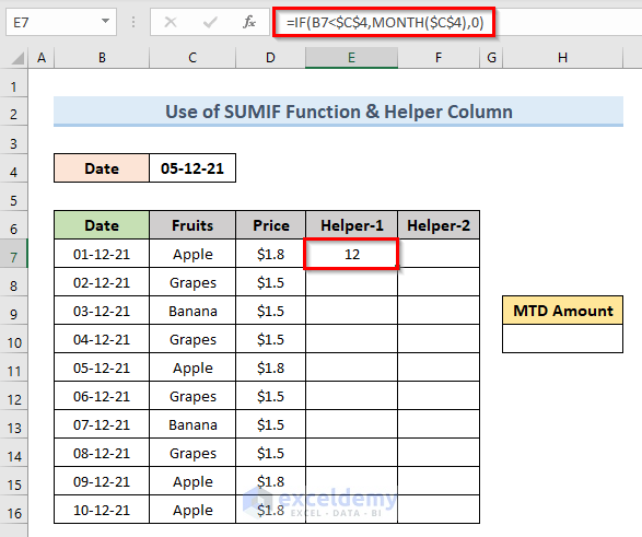
Here, the IF function returns the month number of cell C4 in cell E7 if B7 < C4. Otherwise, the formula will return 0.

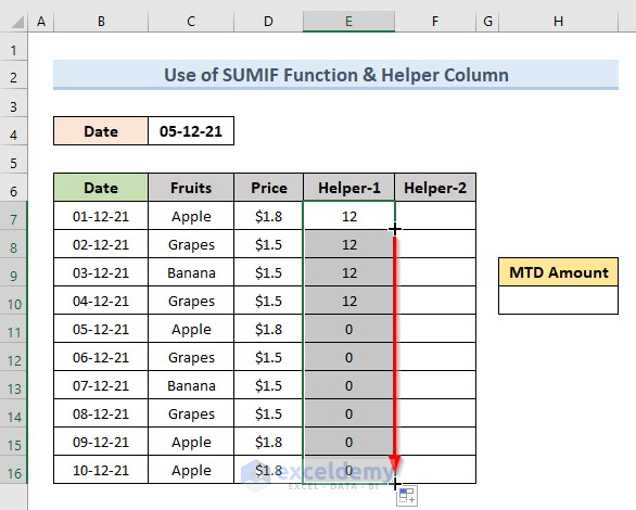
Drag the formula to the end of the dataset and get a result like the following image.

Insert the following formula in cell F7.

=IF(MONTH(B7)=MONTH($C$4),E7,0)

Press Enter.
Drag the Fill Handle to the end of the dataset.

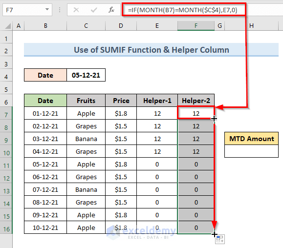
In the above formula, the MONTH function gets the value of the month from the date in cells B7 and C4. It returns the value of cell E7 if the value of B7 and C4 is equal. Otherwise, it will return 0.

Select cell H10 and input the following formula.

=SUMIF($E$7:$E$16,MONTH($C$4),D7:D16)

Hit Enter.

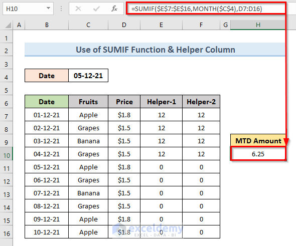
Here, the SUMIF function returns the sum of the range D7:D16. It is valid until the value by the MONTH function in cell C4 remains within the range E7:E16.

NOTE:
If we change the date value in cell C4 the MTD amount will change for the updated date accordingly.

Method 3 – Use Pivot Table & Slicer to Calculate MTD in Excel

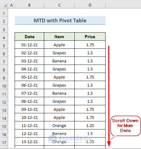
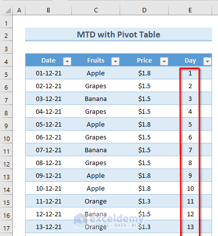
For this, we will use the given dataset of a fruit stall. The dataset includes fruit sales for the 31 days of December 2021 and the 15 days of January 2022.

Steps:

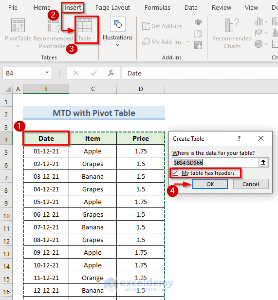
Select any cell from the data range.
Go to Insert > Table.
Check the option My table has headers and click on OK.

Add a new column named Day in the dataset.
Insert the following formula in cell E5.

=DAY(B5)

Press Enter.
Double-click on the Fill Handle icon or drag it to the end of the dataset.

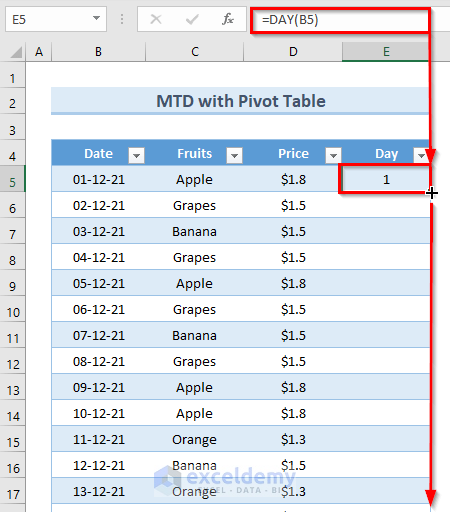
Here the DAY function returns the value of a day from a date field.

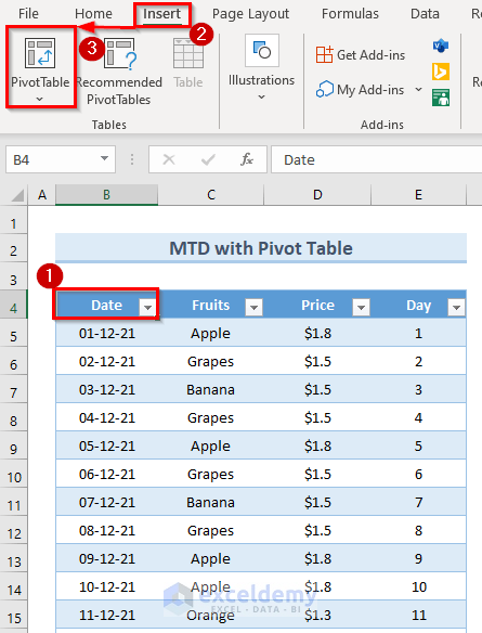
Select any cell from the data range. We have selected cell B4.
Go to the Insert tab and select the option PivotTable.

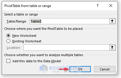
A new dialogue box will open. Click on OK.

A section named PivotTable Fields like the following image will open in a new worksheet.

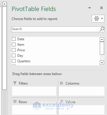
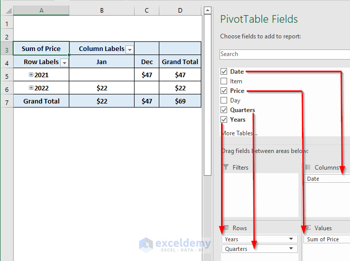
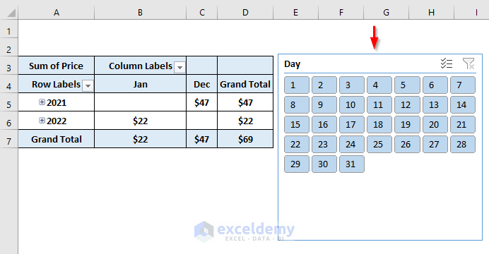
Drag the fields Quarters & Years in the Rows section, Price field in the Value section, and Date field in the Columns section.
We will get results like the below image.

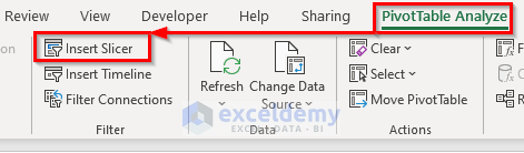
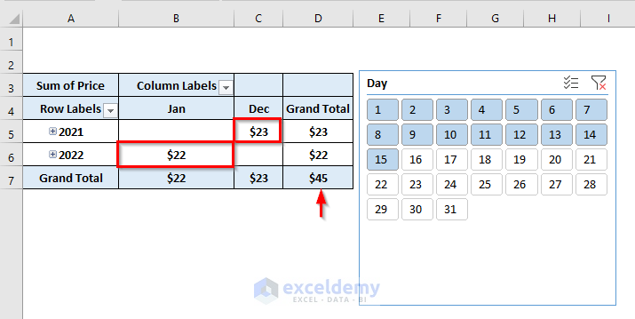
We can’t directly compare the sales amount of months December and January. The result of December month is for 30 days whereas for January it is 15. To compare these two only for 15 days we will add a slicer.
Go to the PivotTable Analyze tab and select the option Insert Slicer.

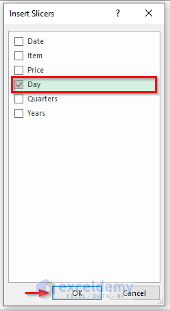
Check the options Day from that dialogue box and click on OK.

We get a slicer for calculating days.

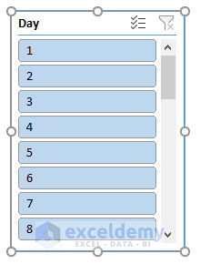
From the Excel ribbon, input the value 7 in the Columns field.

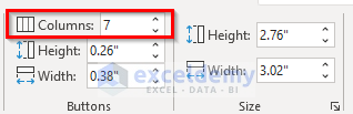
We will get the slicer for 31 days. It will look like a calendar.

Select the first 15 days from the slicer. We can see that the table displays the sales data only for 15 days for both January and December months.