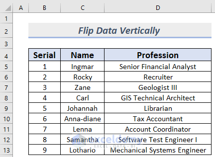
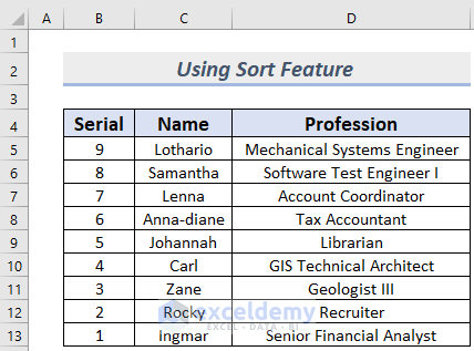
Suppose you have the following dataset:
Method 1 – Combining INDEX and ROWS Functions to Flip Data Vertically in Excel
Steps:
- Make new columns for the newly flipped data.
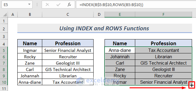
- Type the following formula in the appropriate cell (E5 in this example):
=INDEX(B$5:B$10,ROWS(B5:B$10))
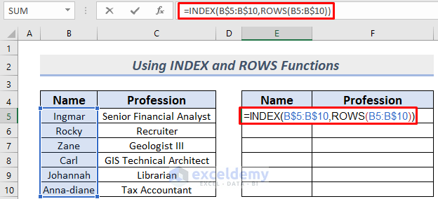
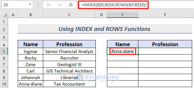
- Press ENTER.
The value from the bottom cell in the column should now show in the top cell.
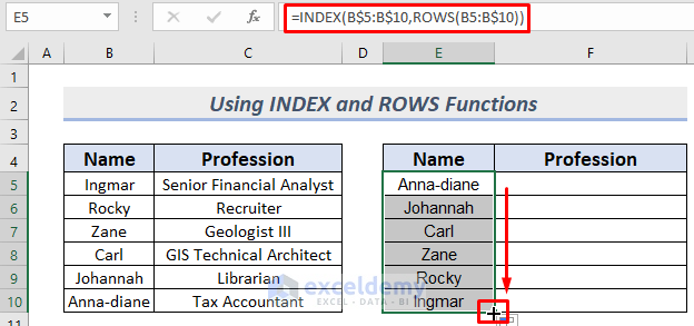
- Use the AutoFill tool to copy the formula to the remaining cells in the column, and then again to the next column as well.
Method 2 – Applying Excel SORTBY and ROW Functions to Vertically Flip Data
Steps:
- Make new columns for the newly flipped data.
- Type the following formula in the appropriate cell (E5 in this example):
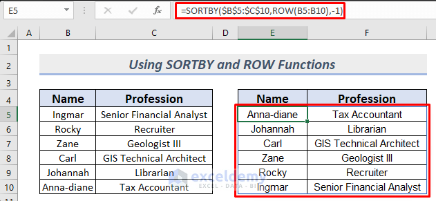
=SORTBY($B$5:$C$10,ROW(B5:B10),-1)
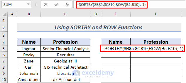
- Press ENTER.
Note: The SORTBY function is only available in the Excel 365 (Office 365) or web versions.
Method 3 – Vertically Flipping Data in Excel with Sort Feature
Steps:
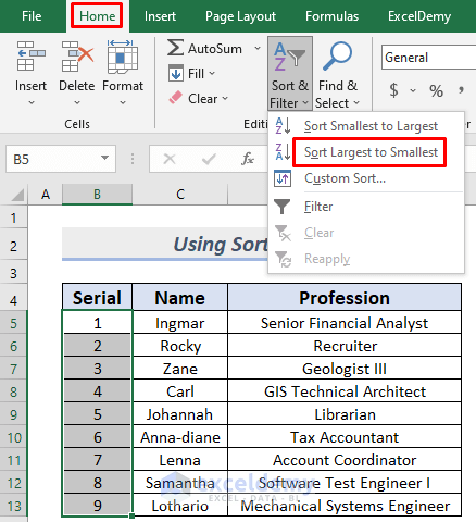
- Select the appropriate cell range (B5 to B10)
- Select Sort & Filter from the Home Ribbon, then choose Sort Largest to Smallest.
- A warning message will pop up.
- Select Expand the selection if appropriate and click on Sort.

The results should be properly flipped.
Method 4 – Using VBA to Flip Data Vertically in Excel
Steps:
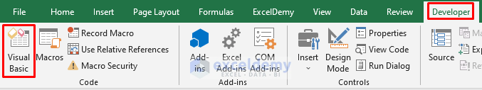
- Go to the Developer Tab and select Visual Basic or press ALT+F11.
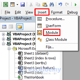
- The VBA editor will appear. Select Insert then Module to open a VBA Module.
- Type the following code in the VBA Module.
Sub FlipDataVertically()
    Dim mn_Cell_Range As Range
    Dim mn_Cell_Array, mn_Temp_Array As Variant
    Dim a1, a2, a3 As Integer
    On Error Resume Next
    Set mn_Cell_Range = Application.InputBox("Select the Range" _
    & " Without Header Row", "ExcelDemy", Type:=8)
    mn_Cell_Array = mn_Cell_Range.Formula
    Application.ScreenUpdating = False
    For a2 = 1 To UBound(mn_Cell_Array, 2)
        a3 = UBound(mn_Cell_Array, 1)
            For a1 = 1 To UBound(mn_Cell_Array, 1) / 2
                mn_Temp_Array = mn_Cell_Array(a1, a2)
                mn_Cell_Array(a1, a2) = mn_Cell_Array(a3, a2)
                mn_Cell_Array(a3, a2) = mn_Temp_Array
                a3 = a3 - 1
            Next
    Next
    mn_Cell_Range.Formula = mn_Cell_Array
    Application.ScreenUpdating = True
End Sub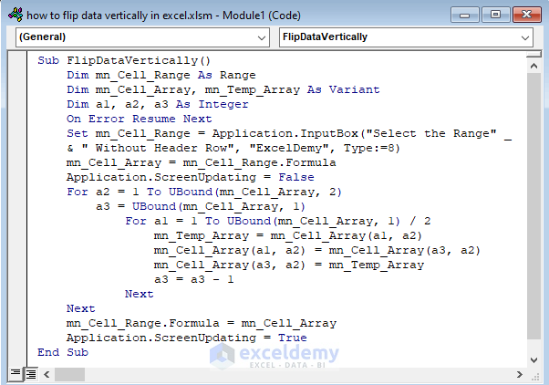
VBA Code Breakdown
- Name the Sub procedure (FlipDataVertically in this example).
- Define the variable types.
- Use the “On Error Resume Next” statement to ignore all the errors.
- Specify the working cell range using the InputBox method.
- For Next Loop is used to loop through the selected cell range.
- Run the code.
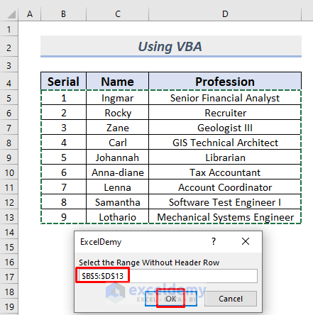
- Go back to the sheet and run the Macro.
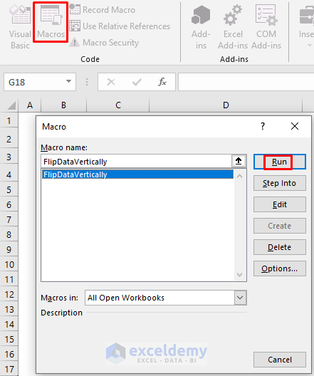
- A message box will appear. Select the range to flip vertically.
- Click OK.
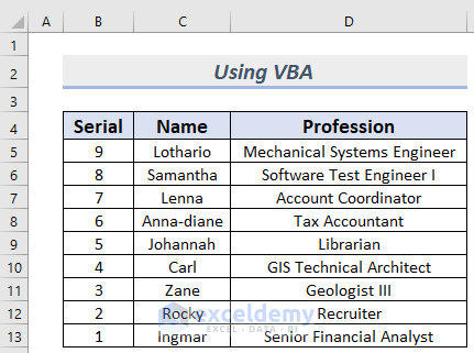
The results should be properly flipped.
Download Practice Workbook
Related Articles
- How to Flip Data Horizontally in Excel
- How to Flip Table in Excel
- How to Flip Data in Excel Chart
- How to Mirror Data in Excel
- How to Reverse Text to Columns in Excel
- How to Reverse Column Order in Excel
- How to Reverse Data in Excel Chart
<< Go Back to Excel Reverse Order | Sort in Excel | Learn Excel
Get FREE Advanced Excel Exercises with Solutions!
