The article will show you how to flip data vertically in Excel. If a user wants to reverse his data so that the data are stored from bottom to top in the Excel sheet, he or she may need to use the feature or formula for flipping data vertically. There are easy methods in Excel to do this. We will be discussing these methods in the later sections of this article.
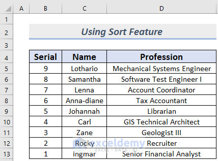
The dataset contains personal information about some folks.
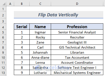
Let’s go through the following sections to see how to flip vertically these data.
1. Combining INDEX and ROWS Functions to Flip Data Vertically in Excel
We will show you how to use the INDEX and ROWS functions to flip data vertically in a dataset in this section. Let’s have a look at the following description for a better understanding. We will not use the Serial column in this example.
Steps:
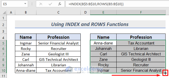
- First, make new columns to store the vertically flipped data and type the following formula in cell E5.
=INDEX(B$5:B$10,ROWS(B5:B$10))
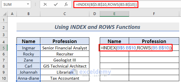
The formula will return the bottom name of column B.
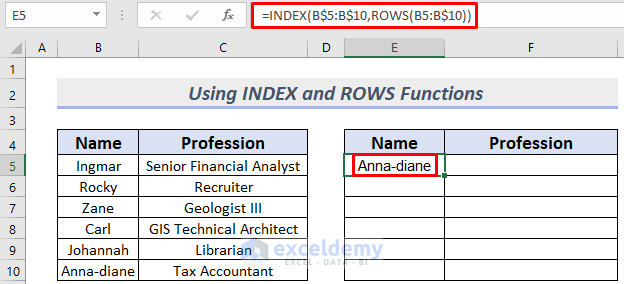
- After that, press the ENTER button and you will see the last name of the dataset in E5 which is Anna-diane.
- Next, use the Fill Handle to AutoFill the lower cells.
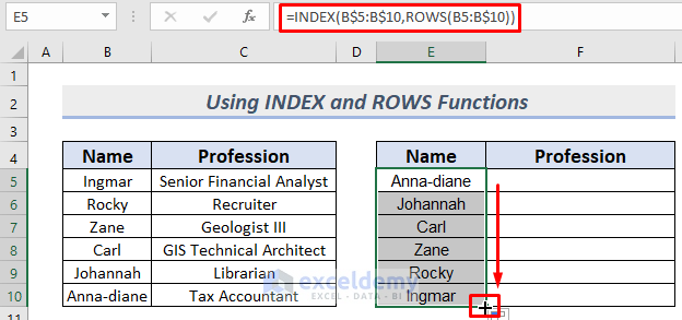
- Thereafter, drag the Fill icon to the right to AutoFill the adjacent column.
Thus you can flip data vertically in Excel using INDEX and ROWS functions.
2. Applying Excel SORTBY and ROW Functions to Vertically Flip Data
We can also use the SORTBY and ROW functions to flip data vertically. The steps of the procedure are given below. We will not use the Serial column in this example.
Steps:
- First, make new columns to store the vertically flipped data and type the following formula in cell E5.
=SORTBY($B$5:$C$10,ROW(B5:B10),-1)
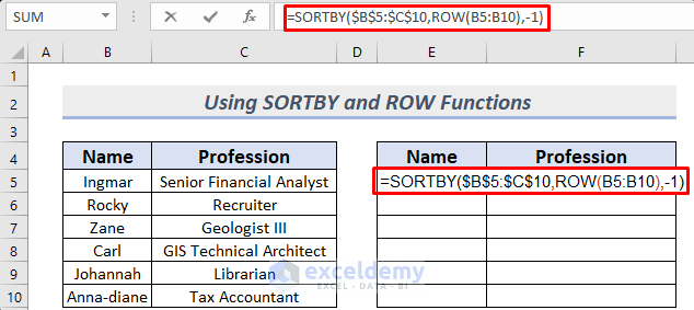
The formula will return an array with the vertically flipped data of the Name and Profession columns.
- After that, hit the ENTER button.
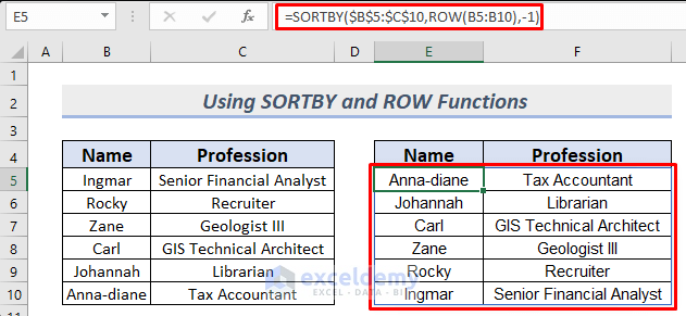
Thus you can flip data vertically in Excel using the SORTBY and ROW functions.
3. Vertically Flipping Data in Excel with Sort Feature
Another way of flipping data vertically in Excel is to apply the Sort feature. We can easily do this by using a column with serial numbers. Let’s go through the process below.
Steps:
- First, select the cells B5 to B10 and then select Home >> Sort & Filter >> Sort Largest to Smallest.
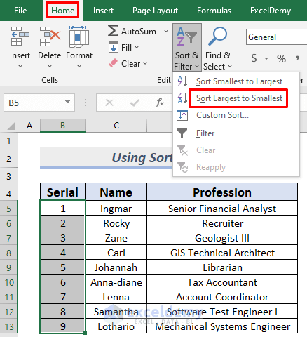
- After that, you will see a warning message. Make sure you select Expand the selection (if you deliberately don’t want to go with only the selected portion) and click on Sort.

There you go, you will see your data flip vertically after this operation.
4. Using VBA to Flip Data Vertically in Excel
We can also use Microsoft Visual Basic for Applications (VBA) to flip Excel data vertically. Let’s see the procedure.
Steps:
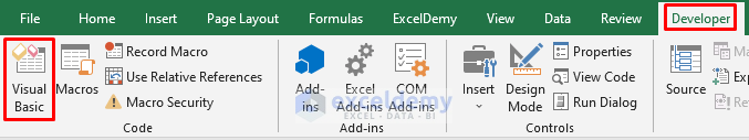
- First, go to the Developer Tab and then select Visual Basic or press ALT+F11.
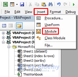
- After that, the VBA editor will appear. Select Insert >> Module to open a VBA Module.
- Now, type the following code in the VBA Module.
Sub FlipDataVertically()
    Dim mn_Cell_Range As Range
    Dim mn_Cell_Array, mn_Temp_Array As Variant
    Dim a1, a2, a3 As Integer
    On Error Resume Next
    Set mn_Cell_Range = Application.InputBox("Select the Range" _
    & " Without Header Row", "ExcelDemy", Type:=8)
    mn_Cell_Array = mn_Cell_Range.Formula
    Application.ScreenUpdating = False
    For a2 = 1 To UBound(mn_Cell_Array, 2)
        a3 = UBound(mn_Cell_Array, 1)
            For a1 = 1 To UBound(mn_Cell_Array, 1) / 2
                mn_Temp_Array = mn_Cell_Array(a1, a2)
                mn_Cell_Array(a1, a2) = mn_Cell_Array(a3, a2)
                mn_Cell_Array(a3, a2) = mn_Temp_Array
                a3 = a3 - 1
            Next
    Next
    mn_Cell_Range.Formula = mn_Cell_Array
    Application.ScreenUpdating = True
End Sub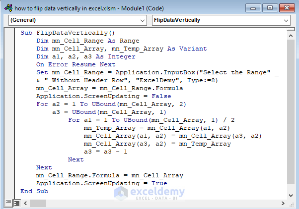
VBA Code Breakdown
- Firstly, we named the Sub procedure FlipDataVertically.
- After that, we defined the variable types.
- Thereafter, we use the “On Error Resume Next” statement to ignore all the errors.
- The user then specifies the working cell range using the InputBox method.
- Next, the For Next Loop is then used to loop through the selected cell range.
- After that, we exchange the rows with the relevant rows to flip them vertically.
- Finally, we run the code.
- After that, go back to your sheet and run the Macro.
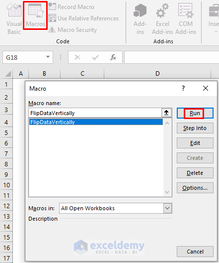
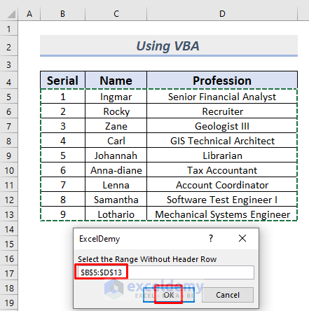
- The execution of this operation will show you a message box, asking you to select the range that you want to flip vertically. Select the range and click OK.
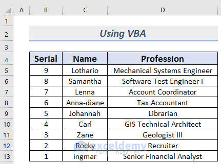
After that, you will see your Excel data flip vertically.
Download Practice Workbook
Conclusion
In the end, hope you will learn the basic ways of how to flip data vertically in Excel after reading this article. If you have any better suggestions or questions or feedback regarding this article, please share them in the comment box. This will help us enrich our upcoming articles and provide you best.
Related Articles
- How to Flip Data Horizontally in Excel
- How to Flip Table in Excel
- How to Flip Data in Excel Chart
- How to Mirror Data in Excel
- How to Reverse Text to Columns in Excel
- How to Reverse Column Order in Excel
- How to Reverse Data in Excel Chart
<< Go Back to Excel Reverse Order | Sort in Excel | Learn Excel
Get FREE Advanced Excel Exercises with Solutions!
