Download Practice Workbook
Download this practice sheet to exercise while you are reading this article.
5 Suitable Methods to Reference to Another Sheet in Excel
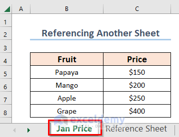
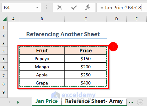
Let’s use a data set on the month of Prices of Fruits in January in a sheet named Jan Price. We will refer to this sheet with another sheet.
Method 1 – Directly Referencing Another Sheet
Steps:
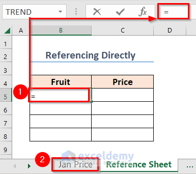
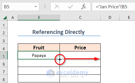
- Select the cell where the formula should go. We are going to use the sheet named Reference Sheet and select cell B5.
- Press the equal sign (=).
- Click on the source sheet (Jan Price).
- Select the cell with data you want to use. We selected cell B5.
- The formula bar is updated.
- Press Enter.
If the source data sheet is named Jan, it will be:
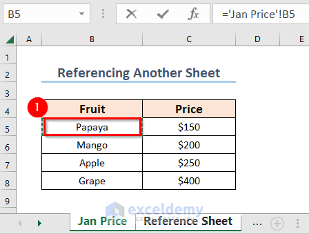
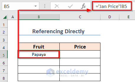
=Jan!B5As our source sheet name contains spaces, then the reference to the sheet will appear in single quotes.
='Jan Price'!B5- If you change the value in the source sheet, then the value of this cell will also change.
- Drag the Fill Handle icon horizontally to C5 to reference the values in the corresponding cells in the source worksheet.
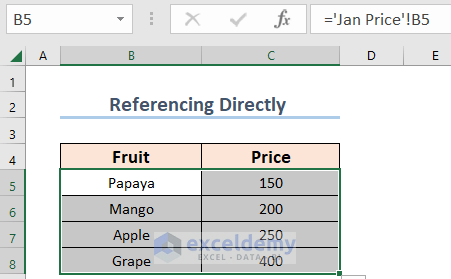
- Drag the Fill Handle icon to paste the used formula to the other cells of the columns.
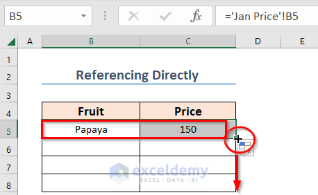
- You will see all the values from the Jan Price sheet.
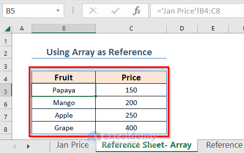
Method 2 – Reference Another Sheet Using an Array Formula
Steps:
- Select a cell in the target sheet Reference Sheet- Array.
- Press the equal sign (=).
- Click on the source sheet (Jan Price).
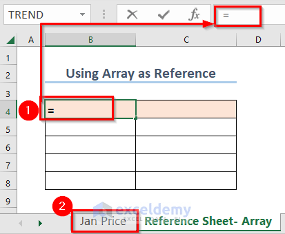
- Select the cells you want to refer to. We will select cells B4 to C8.
- Press Enter.
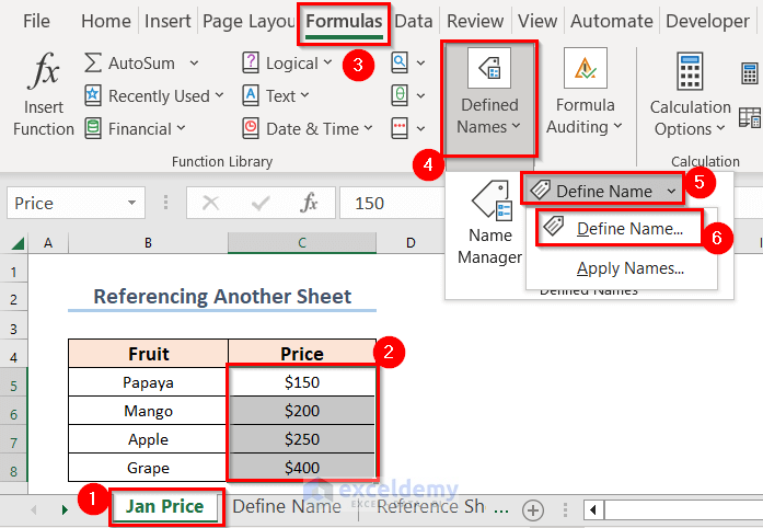
Method 3 – Using the Define Name Feature to Refer to Another Worksheet
Let’s find the total prices for January.
Steps:
- Select the range from the source data.
- From the Top Ribbon, go to the Formulas bar and click on Defined Names.
- From the drop-down, select Define Name and a new drop-down will appear.
- From the last drop-down, select Define Name.
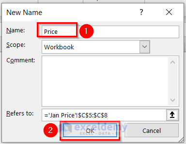
- You will get a pop-pp named New Name.
- In the Name box put a name, which will be the array’s reference name in the future. Here, we put Price as the name.
- Press OK.
The range names must be unique.
- Go to your target sheet and input the SUM function.
- In the SUM function, when you write “Pr”, you will get some recommended options. Choose Price.
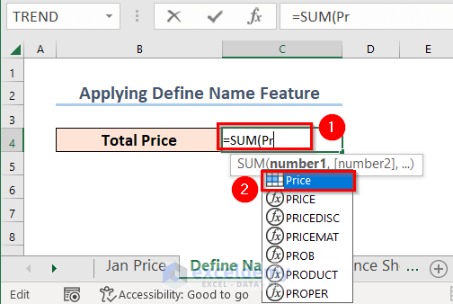
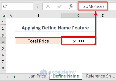
- Here’s the formula you can copy:
=SUM(Price)- Press Enter to get the sum of the selected range.
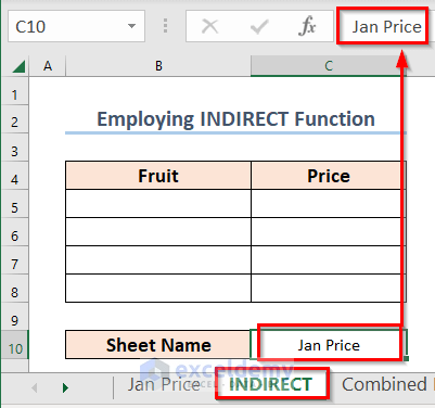
Method 4 – Use the INDIRECT Function for Calling Another Sheet in Excel
Steps:
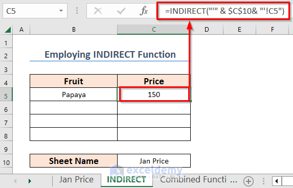
- Write the sheet name in a cell. We put the name in a new cell C10.
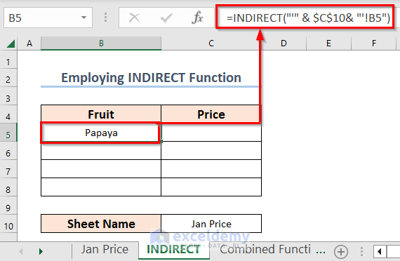
- Select another cell B5 where you want to get the Fruits.
- Use the formula given below in B5:
=INDIRECT("'" & $C$10& "'!B5")- Press Enter to get the result.
Formula Breakdown
- First, $C$10 returns the value of the C10 cell. Which is Jan Price. Actually, the Dollar sign will freeze the C10 position for other cells too.
- The Single Quote or Apostrophe (‘) is required for using any strings or signs.
- The Ampersand sign (&) will join all these terms.
- INDIRECT(“‘” & $C$10& “‘!B5”)—> becomes
- INDIRECT(‘Jan Price’!B5). Which will return the value of B5 from the Jan Price sheet.
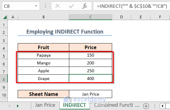
- Copy the following formula to C5.
=INDIRECT("'" & $C$10& "'!C5")- Press Enter.
We have to manually change the corresponding cell references that contain Fruit or Price data. The sheet name is fixed for all the cells so we used the Dollar sign ($) for it.
- Write the same formula, changing the cell reference for the other cells.
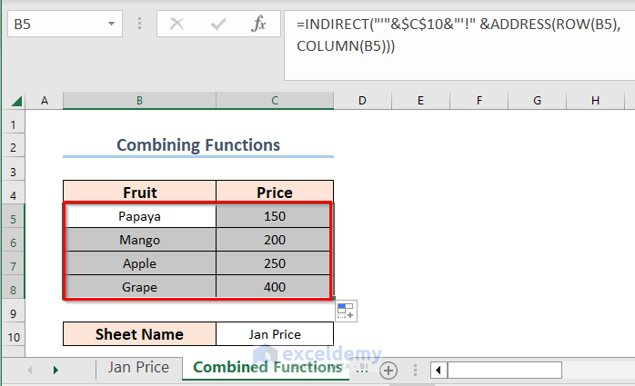
Method 5 – Combine INDIRECT, ADDRESS, ROW, and COLUMN Functions
Steps:
- Write the sheet name in a cell. We put that in cell C10.
- Use the formula given below in a blank cell B5.
=INDIRECT("'"&$C$10&"'!" &ADDRESS(ROW(B5),COLUMN(B5)))- Press Enter to get the result.
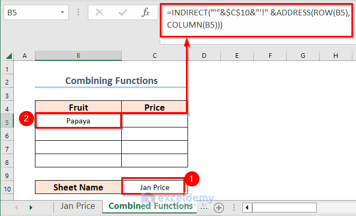
Formula Breakdown
- ROW(B5)→ returns the row number of the cell B5.
- Output→ 5.
- COLUMN(B5)→ returns the column number of the cell B5.
- Output→ 2.
- ADDRESS(ROW(B5),COLUMN(B5)) becomes ADDRESS(5,2).
- Output→ $B$5.
- Lastly, the Ampersand sign (&) will join all these terms.
- INDIRECT(“‘”&$C$10&”‘!” &ADDRESS(ROW(B5),COLUMN(B5))) becomes INDIRECT(“‘”&$C$10&”‘!” &$B$5)→INDIRECT(‘JanPrice’!$B$5).
- Output→ Papaya.
- Drag the Fill Handle icon horizontally to cell C5.
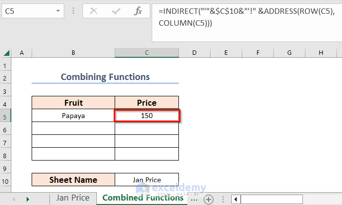
- Drag the Fill Handle vertically to fill the rest of the dataset.
Practice Section
You can practice these methods in the workbook we provided at the start of the article.
Reference to Another Sheet: Knowledge Hub
<< Go Back to Cell Reference in Excel | Excel Formulas | Learn Excel
Get FREE Advanced Excel Exercises with Solutions!
