While working with Excel, we sometimes need to share files with others. Whenever the file is distributed with other authors and users, it allows the user to hide their work. Only by securing the locked cells can you completely prevent the user from altering them. By encrypting the spreadsheet with a passcode, we can prevent others from altering the data fields. In this article, we will demonstrate some effective ways to protect formulas without protecting the worksheet in Excel.
Individuals can safeguard the content of any Excel document with a passcode to restrict other users from reading hidden spreadsheets, editing, relocating, removing, concealing worksheets, or rearranging spreadsheets. However, the formula in the selected cell will appear in the formula bar.
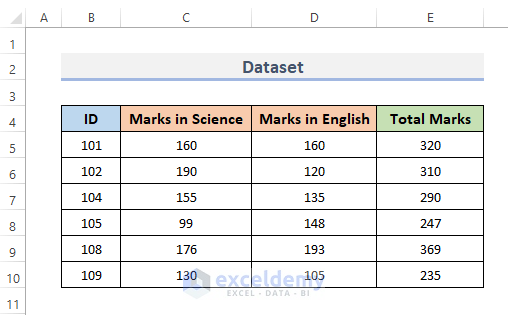
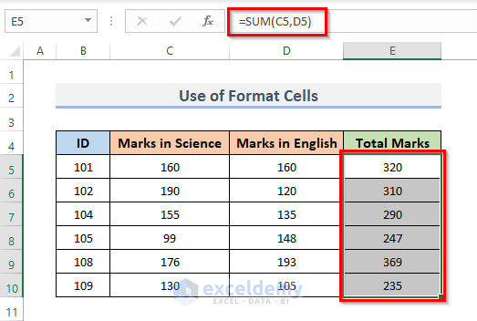
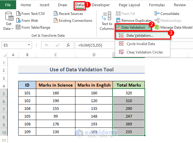
Suppose, we have a dataset containing some student ID in column B, Marks in Science in column C (out of 200), Marks in English in column D (out of 200), and the Total Marks in column E (out of 400). To obtain the total marks, we use the SUM function in cell E5. We use the formula below.
=SUM(C5,D5)And, we want to protect the cell range E5:E10, containing the formula.
1. Using Format Cells Feature to Protect Formulas Without Protecting Excel Worksheet
Just the appearance of cell data in the worksheet can be changed with the Format Cells. It is vital to remember that this just changes the way the data is displayed, not the usefulness of the information. We can protect formulas without protecting worksheets using Format Cells. For this, we need to follow some procedures down.
STEPS:
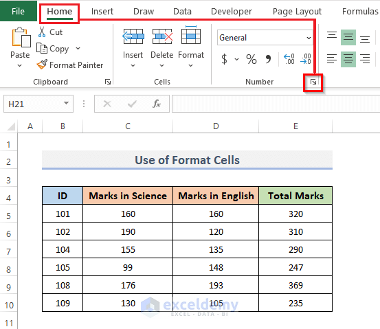
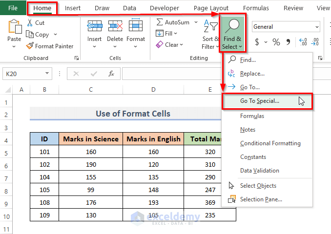
- Firstly, go to the Home tab from the ribbon.
- Secondly, to open the Format Cells feature, on the Number group, click on the tiny icon shown in the screenshot.
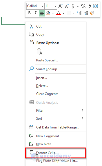
- Instead of doing this, right-click on your mouse then, select Format Cells.
- Alternatively, press the Ctrl + 1 key on your keyboard.
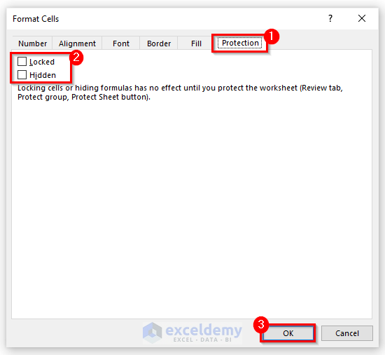
- This will display the Format Cells dialog box.
- Now, click on the Protection menu then, uncheck the Locked and Hidden checkbox.
- Further, click OK to continue the process.
- Furthermore, again go to the Home tab on the ribbon.
- Next, click on Find & Select drop-down menu, under the Editing category.
- Then, click on Go To Special.
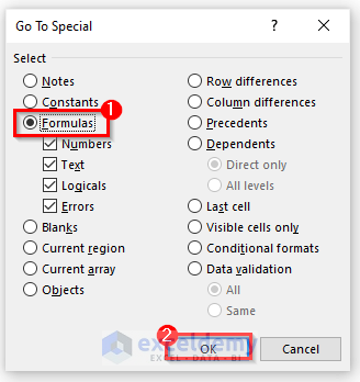
- This will appear in the Go To Special dialog.
- After that, choose the Formulas option from the Select option box.
- Click on the OK button to close the dialog.
- This will automatically select the cells containing the formula and the formula will show in the formula bar.
- Here, we again have to open the Format Cells.
- Likewise, in the previous step, click the little icon displayed to open the Format Cells feature in the Number group.
- Instead, right-click on your mouse and pick Format Cells from the drop-down menu.
- Otherwise, you can use the Ctrl + 1 key combination on your keyboard.
- Go to the Protection menu on the Format Cells dialog box.
- Check the box next to the Locked option. Click OK.

- Go to the Review tab from the ribbon, and select the formulated cells.
- From the Protect category, click on Protect Sheet.

- This will open the Protect Sheet dialog.
- Type the password that you put earlier on the Password to unprotect sheet.
- Make sure that Select locked cells and Select unlocked cells are checked.
- Click OK.

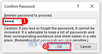
- A Confirm Password popup will display once again to verify that the password you are entering is accurate.
- Finally, click OK.
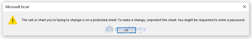
- If you want to edit the formulated cells, an error message will appear.
- By following those steps, we can easily protect formulas without protecting worksheets.
2. Protecting Formulas Without Protecting Worksheet Through Data Validation Tool
Excel may utilize data validation to limit data input to specific cells, ask users to submit actual information whenever a cell is picked, and display an error message if they enter incorrect information. Data validation is an Excel feature that restricts what users can type into a cell. It enables us to establish customized rules. We can use the Data Validation tool to protect formulas without protecting worksheets. For this, we need to follow some steps to complete the work.
STEPS:
- In the first place, go to the Home tab from the ribbon.
- Next, under the Editing category, select Find & Select from the drop-down menu.
- Select Formula From the drop-down menu.

- This will pick the cells that contain the formula and display the formula in the formula bar.
- Further, go to the Data tab on the ribbon.
- Then, from the Data Tools group, click on the Data Validation drop-down menu and select Data Validation.
- Alternatively, use the keyboard shortcut Alt + D + L to open the Data Validation dialog.
- Now, we can see the Data Validation dialog.
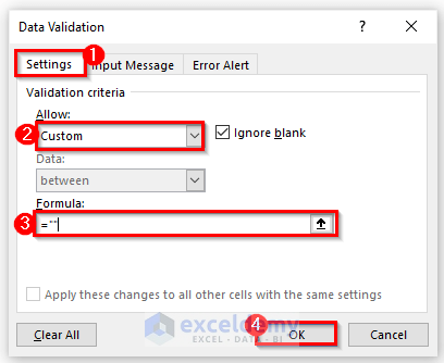
- Further, click on the Settings menu from the dialog.
- From the Allow drop-down menu, select Custom.
- In the Formula box, type (=“”).
- Click OK to close the dialog.
- If we put content in the cell, the formula will not alter and a pop-up will display.

- And that is how we can use data validation in Microsoft Excel to protect formulas without protecting worksheets.
Read More: How to Protect Formula in Excel but Allow Input
3. Applying Excel VBA to Protect Formulas Without Protecting Worksheet
With Excel VBA, users can easily use the code which acts as Excel menus from the ribbon. To use the VBA code to protect formulas without protecting worksheets, let’s follow the procedure.
STEPS:
- Firstly, go to the Developer tab from the ribbon.
- Secondly, from the Code category, click on Visual Basic to open the Visual Basic Editor. Or press Alt + F11 to open the Visual Basic Editor.

- Instead of doing this, you can just right-click on your worksheet and go to View Code. This will also take you to Visual Basic Editor.

- This will appear in the Visual Basic Editor where we write our codes to create a table from range.
- And, copy and paste the VBA code shown below.
VBA Code:
Sub ProtectFormula()
For Each r In ActiveSheet.Range("B5:E10")
    If r.HasFormula Then
        r.Locked = True
    Else
        r.Locked = False
    End If
Next r
ActiveSheet.Protect "pass"
End Sub- After that, run the code by clicking on the RubSub button or pressing the keyboard shortcut F5.

You don’t need to change the code. All you can do is just change the range as per your requirements.
- If you try to edit the formulated cells now, you’ll get an error notice in Excel.
- By using the following Excel VBA code, we can protect formulas without protecting worksheets.
Download Practice Workbook
You can download the workbook and practice with them.
Conclusion
The above methods will assist you in Protect Formulas Without Protecting Worksheets in Excel. Hope this will help you! If you have any questions, suggestions, or feedback please let us know in the comment section.
Related Articles
<< Go Back to Excel Protect Formulas | Excel Formulas | Learn Excel
Get FREE Advanced Excel Exercises with Solutions!

Hi – I love the second solution, but I did it within a table, and now I am getting the little green flag errors on every cell with a formula when a new row gets added. Any idea if there is a fix for this other than turning of the error checking? It is a shared file so I can’t do that for everyone. Thanks!
Hello, LIZ!
Thanks for sharing your problem with us!
Excel automatically detects all difficulties when you interact with it, including inaccurate data in the cell, issues with formulae, etc. As a result, the top left corner of these cells is shown (by default) with green triangles. Excel displays green triangles, this green triangle indicates a potential mistake, although it is frequently ineffective.
Do the following to disable these green triangles or automatic calculation checks:
1. Go to the File tab from the ribbon.
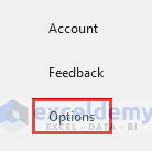
2. Select the Options option from the File tab.
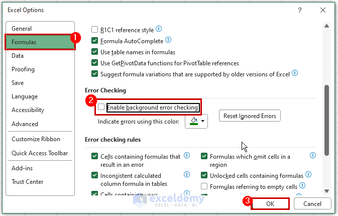
3. Enable background error checking is an option that may be disabled in the Excel Options dialog box’s Formulas tab’s Error Checking section.
All open workbooks in the Excel session will be affected by this application-level option.
Hope this will help you!
If not, can you please send me your excel file via email? ([email protected]).
Good Luck!
Best Regards
Sabrina Ayon
Author, ExcelDemy.