[Fixed!] FORECAST Function Not Accurate in Excel (5 Solutions)

Undoubtedly, Excel’s forecasting functions are very useful since they can predict future output based on past results. However, like everything else in this world, there are downsides too. Have you faced a situation where the FORECAST function returns invalid results? Do not despair! Because you’re not alone. Luckily, in the following tutorial, we’ll demonstrate 5 fixes for the FORECAST function not accurate in Excel. In addition, we’ll also discuss how to apply the FORECAST function with seasonality in Excel.

How to Fix Accuracy of FORECAST Function in Excel: 5 Ways

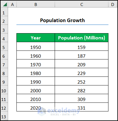
First of all, let’s suppose the Population Growth dataset in the B4:C12 cells contains the “Year” and “Population (Million)” columns respectively. Here, we want to apply this dataset to fix the accuracy of the FORECAST function in Excel, so let’s see each of the problems and solutions in the methods below.

Here, we have used the Microsoft Excel 365 version; you may use any other version at your convenience.

1. Correcting Reversed X and Y Arguments

First and foremost, a common cause of the FORECAST function not being accurate in Excel is due to the mix-up of the X and Y arguments, resulting in the wrong output.

📌 Steps:

• In the first place, the formula in the C16 cell shows the incorrect output.

Here, the arguments for the Horizontal (X) and Vertical (Y) series have been swapped which causes inaccurate results.

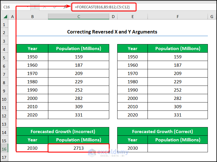
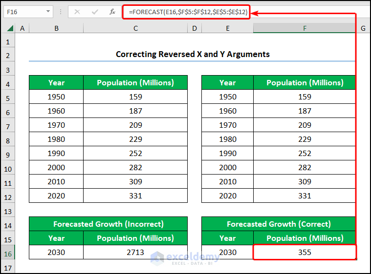
• Next, go to the F16 cell >> enter the correct formula given below to get the proper answer.

For example, the E16 cell represents the X value (“2030”), in contrast, the E5:E12 and F5:F12 arrays point to the known values of X and Y respectively.

2. Anchoring Cells

For instance, another minor problem that drives people crazy is when they forget to Anchor the cells and then use the Fill Handle tool to obtain incorrect results.

📌 Steps:

• In this scenario, the expression in the C16 cell is not anchored, so using the Fill Handle tool shifts the B5:B12 and C5:C12 ranges.

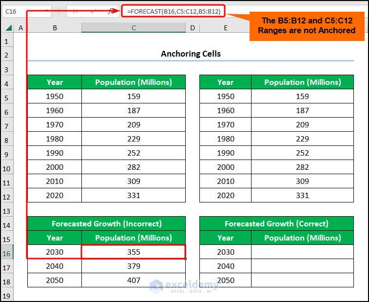
• Now, to correct the wrong, move to the F16 cell >> copy and paste the following formula >> then use the Fill Handle to copy the formula to the cells below.

Read More: TREND vs FORECAST Function in Excel

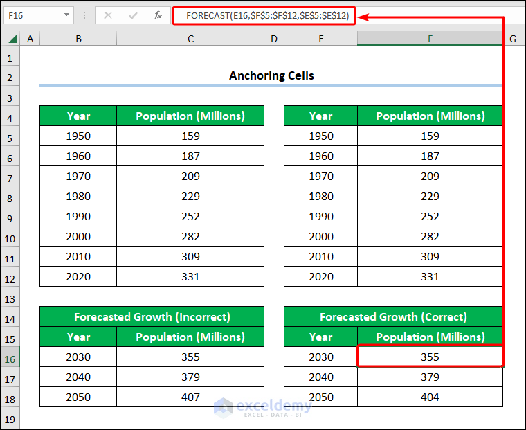
3. Checking Non-Numeric Values

Alternatively, we have to ensure that there are no text values instead of numeric values, otherwise, the function returns an error.

📌 Steps:

• Clearly, the FORECAST function is showing the #DIV/0! error (division by zero).

Here, the value in the B16 cell is formatted as text.

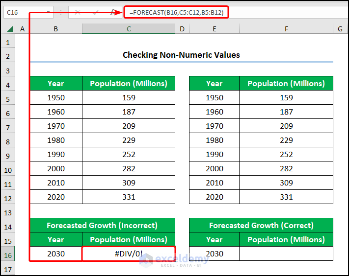
• Here, the leading Apostrophe (‘) comma causes the function to consider the “2030” value as a string of text.

• Following this, use the equation below >> make sure to check that the value in the E16 cell is numeric.

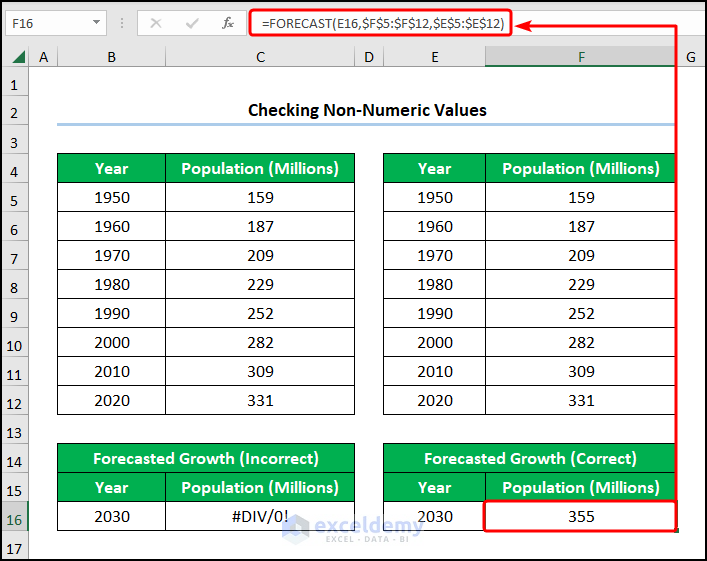
4. Choosing Correct Range

Besides, it is also possible that we may select the incorrect time series range when using the FORECAST function.

📌 Steps:

• To clarify, in the picture below, the range B4:B12 is causing the #N/A error (not available) since it contains the column heading “Year”.

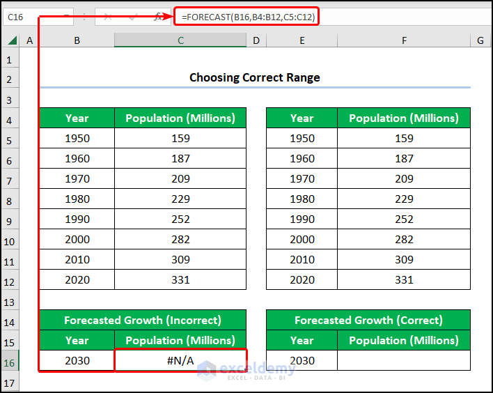
• Rather, we have to enter the correct range which is given in the formula below.

Read More: How to Use VBA Forecast Function in Excel

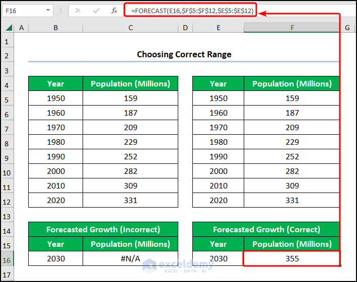
5. Selecting Correct Value of X

For one thing, Excel’s FORECAST function displays a #VALUE! error if the X value is a text.

📌 Steps:

• Indeed, the B15 cell in the formula below refers to the column heading “Year”.

• Nonetheless, the corrected expression is provided below where the E16 cell indicates the value “2030”.

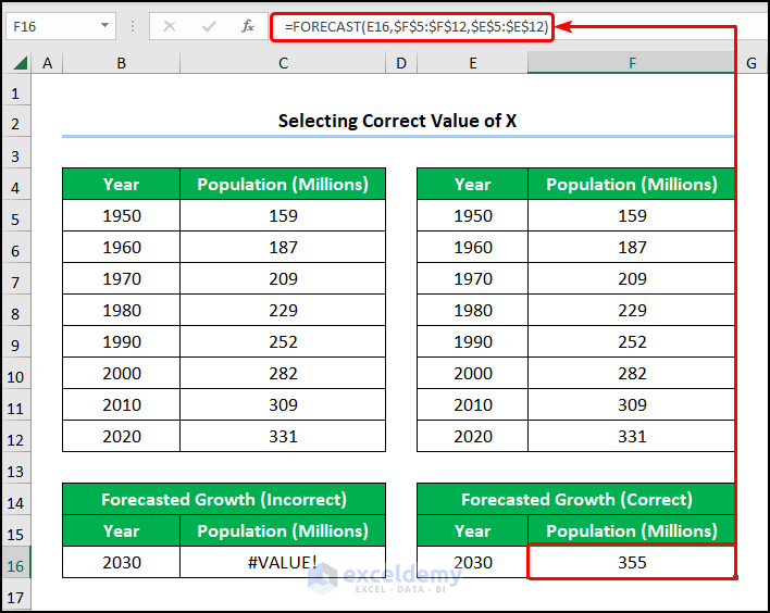
All said and done, the world we live in is far from perfect! Though the methods above are all possible ways to resolve the FORECAST function not being accurate in Excel, if the problem persists as the last option, you can contact Microsoft Support. Here, you can find many Excel experts who will provide solutions for your particular issues.

Read More: How to Use FORECAST Function with Multiple Variables in Excel

How to Apply FORECAST Function with Seasonality in Excel

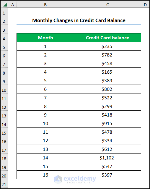
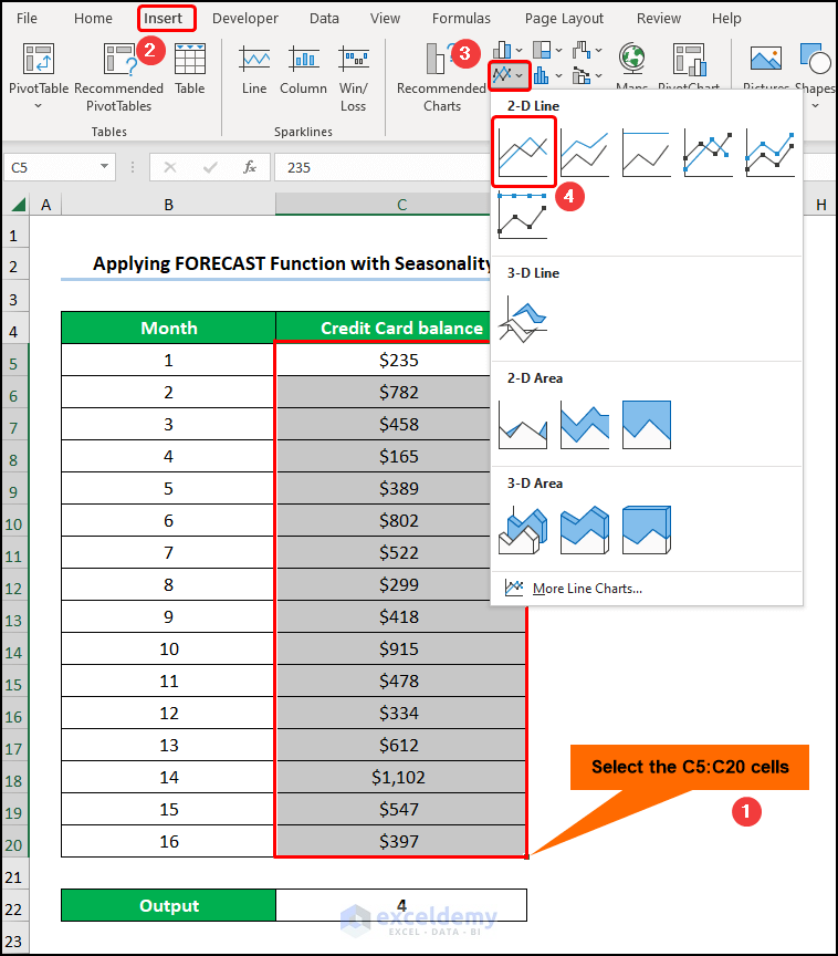
Last but not least, we can apply the FORECAST function with seasonality to compute the timeline of a repetitive pattern. In this situation, we’ll consider the Monthly Changes in Credit Balance dataset which contains the “Month” and “Credit Card Balance” columns respectively.

📌 Steps:

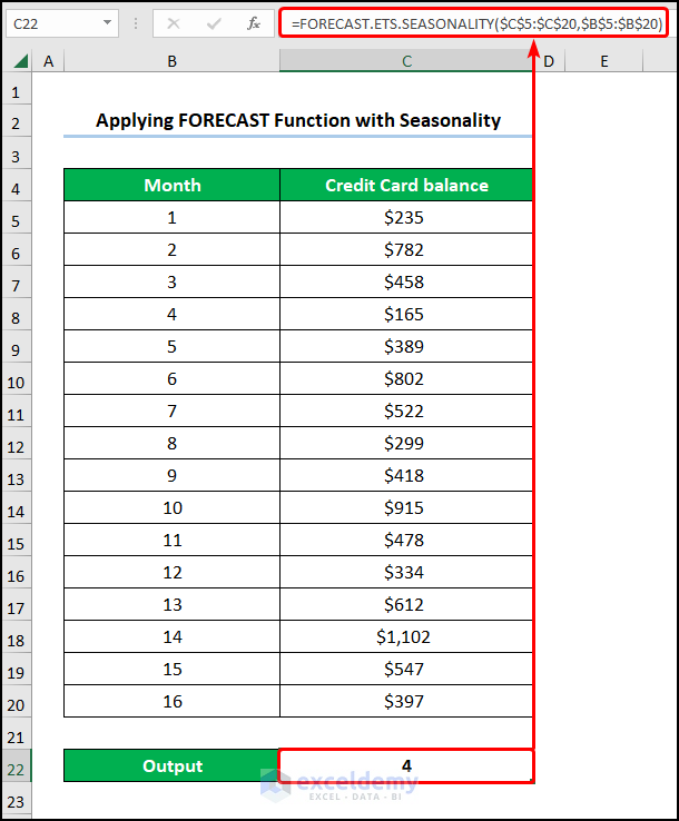
• First, proceed to the C22 cell >>  enter the formula given below.

In this case, the B5:B20 and C5:C20 range of cells indicate the “Month” and “Credit Card Balance” columns respectively.

• Second, select the C5:C20 array >> navigate to the Insert tab >> click the Insert Line or Area Chart option >> choose the Line Chart option.

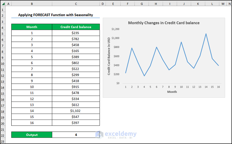
• Third, format the chart using the Chart Elements option.
  • In addition to the default selection, you can enable the Axes Title to provide axes names. Here, it is the “Month” and the “Credit Card Balance in USD”.
  • Now, add the Chart Title, for example, “Monthly Changes in Credit Card Balance”.
  • Lastly, you can disable the Gridlines option to give your chart a clean look.

Eventually, this should generate the chart as shown in the picture below.

Download Practice Workbook

Conclusion

To sum up, we hope this tutorial has provided you with helpful knowledge on the fixes for the FORECAST function not accurate in Excel. Now, we recommend you apply all this know-how in the practice dataset by downloading the practice workbook. In addition, feel free to comment and provide your valuable feedback.