Method 1 – Using the FORECAST Function
- Enter the following formula in cell C12.
=FORECAST(B12, C5:C11, B5:B11)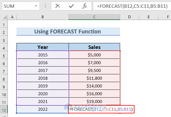
Formula Breakdown
- FORECAST(B12, C5:C11, B5:B11) → The FORECAST function determines the future value based on a current value.
- B12 → Current value of the Year (2022).
- C5:C11 → Known range of Y values (Sales).
- B5:B11 → Known X value (Years).
- Output: $20971
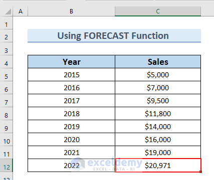
- Press ENTER.
- Cell C12 will display the result: $20971.
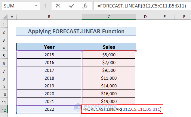
Method 2 – Using the FORECAST.LINEAR Function
- Enter the following formula in cell C12.
=FORECAST.LINEAR(B12,C5:C11,B5:B11)
Formula Breakdown
- LINEAR(B12,C5:C11,B5:B11) → the FORECAST.LINEAR function determines the future value based on a current value.
- B12 → Current value of the Year (2022).
- C5:C11 → Known range of Y values (Sales).
- B5:B11 → Known X value (Years)
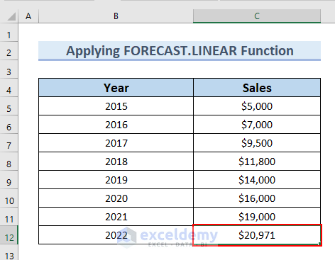
- Output: $20971
- Press ENTER.
- You can see the result in cell C12.
Method 3 – Using the FORECAST.ETS Function
- Enter the following formula in cell C12.
=FORECAST.ETS(B12,C5:C11,B5:B11)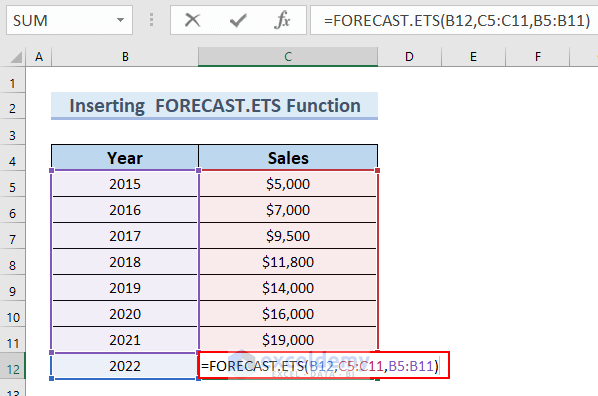
Formula Breakdown
- ETS(B12,C5:C11,B5:B11) → the FORECAST.ETS function determines the future value based on existing historical value.
- B12 → Target_date (2022).
- C5:C11 → Historical values.
- B5:B11 → Timeline (known years).
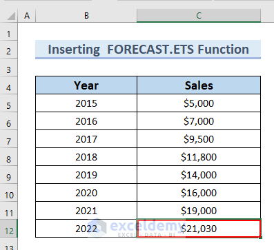
- Output: $ 21030
- Press ENTER.
- You can see the result in cell C12.
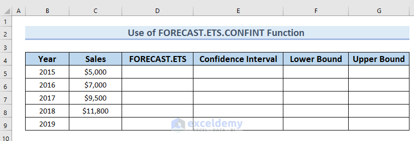
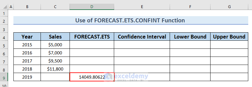
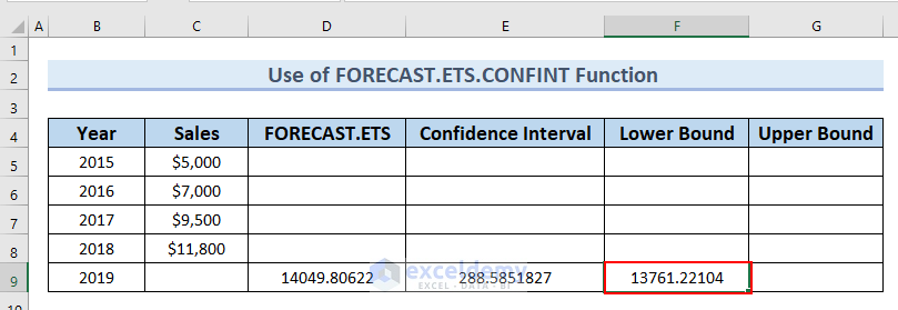
Method 4 – Using the FORECAST.ETS.CONFINT Function
The following dataset contains the Year and Sales values. However, the sales for the year 2019 are missing.
- We will use FORECAST.ETS function to determine FORECAST.ETS for the year 2019.
- We will use the FORECAST.ETS.CONFINT function to determine Confidence Interval.
- We will determine Lower Bound and Upper Bound.
- Enter the following formula in cell D9.
=FORECAST.ETS(B9, C5:C8, B5:B8)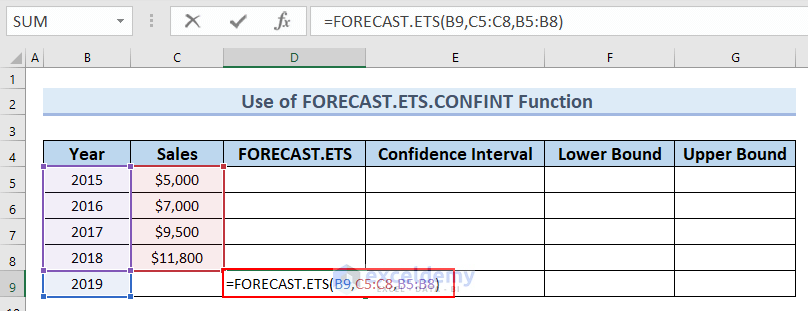
- Press ENTER.
- You can see the result in cell D9.
- To determine the Confidence Interval, enter the following formula in cell E9.
=FORECAST.ETS.CONFINT(B9,C5:C8,B5:B8)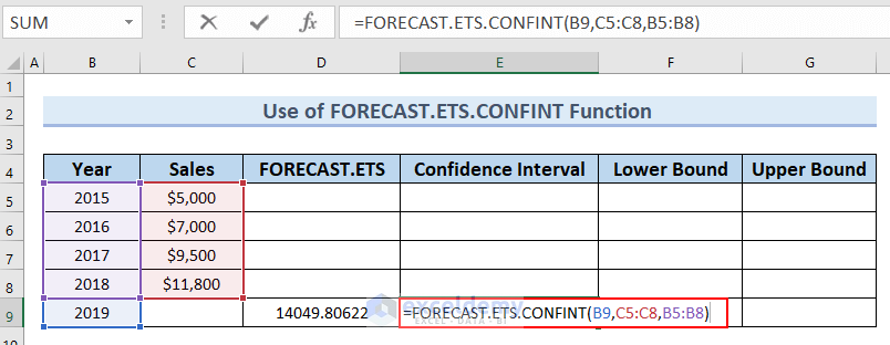
Formula Breakdown
- ETS.CONFINT(B9, C5:C8, B5:B8) → determines the Confidence Interval for a forecast value at a specified target date.
- B9 → Target_date.
- C5:C8 → Historical values.
- B5:B8 → Timeline.
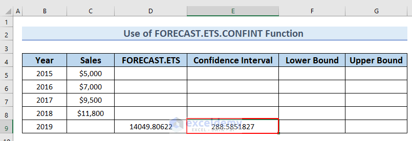
- Output: 288.5851827
- Press ENTER.
- You can see the Confidence Interval for the Year 2022 in cell E9.
- To find out the Lower Bound, enter the following formula in cell F9.
=D9-E9This subtracts the Confidence Interval from FORECAST.ETS value.
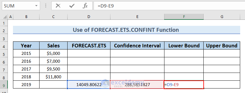
- Press ENTER.
- You can see the Lower Bound in cell F9.
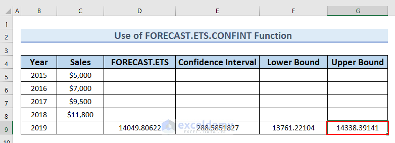
- To determine the Upper Bound, enter the following formula in cell G9.
=D9+E9This adds the Confidence Interval from FORECAST.ETS value.
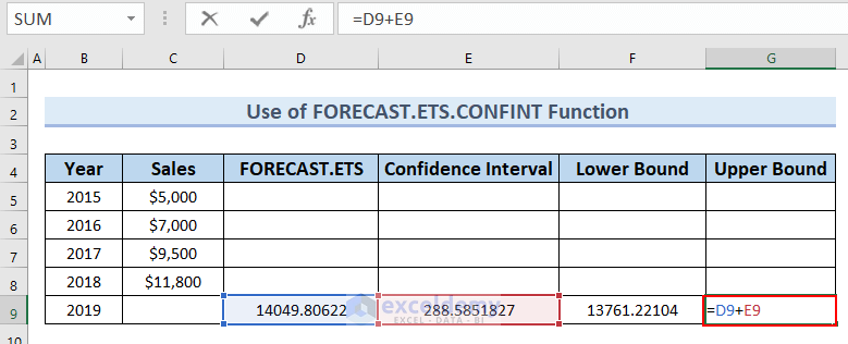
- Press ENTER.
- You can see the Upper Bound in cell G9.
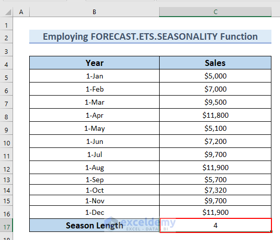
Method 5 – Using the FORECAST.ETS.SEASONALITY Function
- Enter the following formula in cell C17.
=FORECAST.ETS.SEASONALITY(C5:C16,B5:B16,1,1)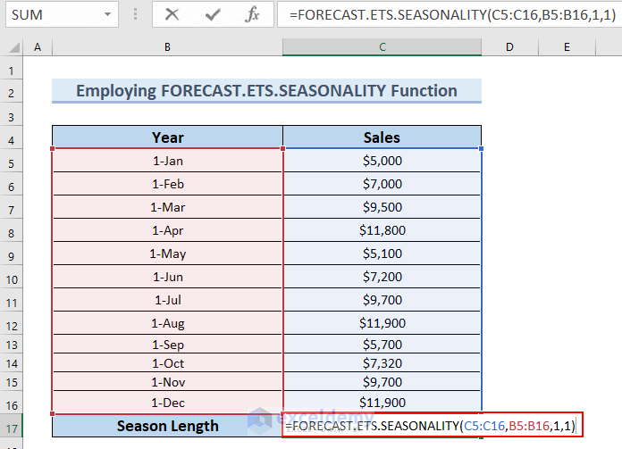
Formula Breakdown
- ETS.SEASONALITY(C5:C16, B5:B16,1,1) → determines the Season Length for specific repetitive time length.
- C5:C16 → Historical values.
- B5:B16 → Timeline.
- 1 → Data Completion
- 1 → Aggregation
- Output: 4
- Press ENTER.
- The result will display in cell C17.
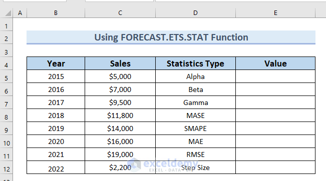
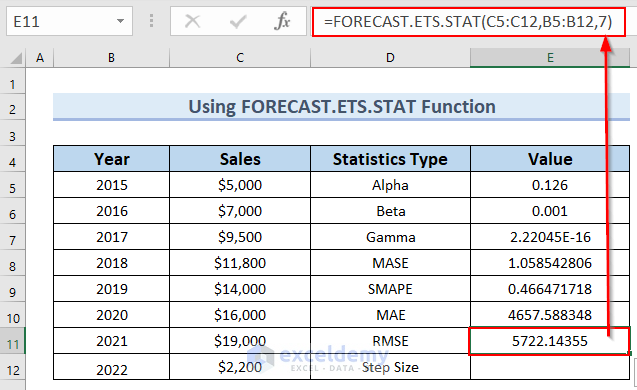
Method 6 – Using FORECAST.ETS.STAT Function
We have 8 statistical argument types:
- Alpha (base value): Smoothing value between 0 and 1, controlling data point weighting.
- Beta (trend value): Determines trend calculation (higher value gives more weight to recent trends).
- Gamma (seasonality value): Controls ETS forecast seasonality (increasing value emphasizes recent seasonal periods).
- MASE (mean absolute scaled error): Evaluates forecast accuracy.
- SMAPE (symmetric mean absolute percentage error): Measures accuracy based on error proportion.
- MAE (mean absolute error): Calculates average forecast error size (independent of direction).
- RMSE (root mean square error): Evaluates discrepancies between observed and projected values.
- Step size detected: Detected timeline step size.
We will determine the Value of these argument types.
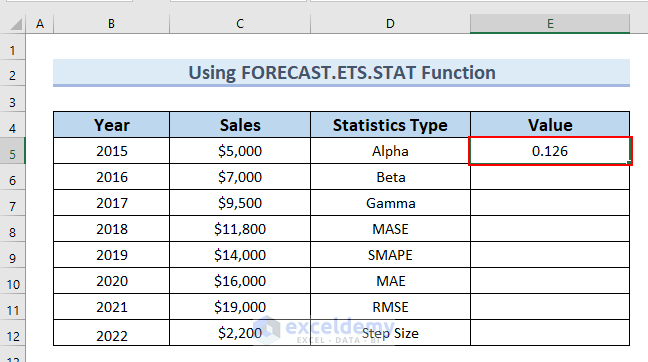
- To find the value of Alpha, enter the following formula in cell E5.
=FORECAST.ETS.STAT(C5:C12,B5:B12,1)
Formula Breakdown
- ETS.STAT(C5:C12,B5:B12,1) → the FORECAT.ETS.STAT function returns the statistical value.
- C5:C12 → Historical values.
- B5:B12 → Timeline.
- 1 → The Statistics_type which is Alpha in that case.
- Output: 0.126
- Press ENTER.
- You can see the output in cell E5.
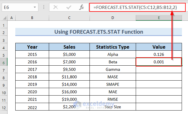
- To determine the Beta value, enter the following formula in cell E6.
=FORECAST.ETS.STAT(C5:C12, B5:B12,2)- Press ENTER.
- You can see the result in cell E6.
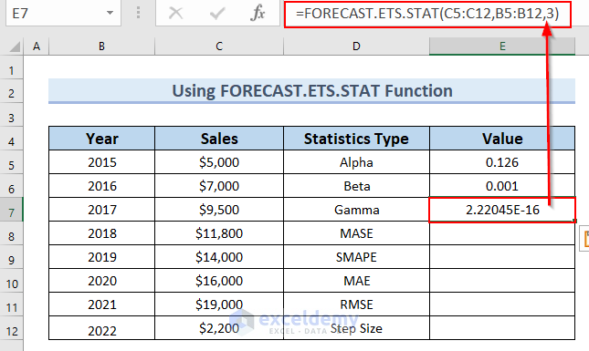
- To calculate the Gamma value, enter the following formula in cell E7.
=FORECAST.ETS.STAT(C5:C12, B5:B12,3)- Press ENTER.
- You can see the result in cell E7.
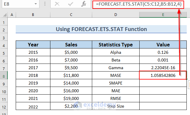
- To find out the MASE value, enter the following formula in cell E8.
=FORECAST.ETS.STAT(C5:C12, B5:B12,4)- Press ENTER.
- You can see the result in cell E8.
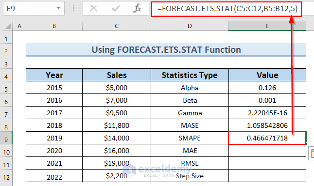
- To determine the SMAPE value, enter the following formula in cell E9.
=FORECAST.ETS.STAT(C5:C12, B5:B12,5)- Press ENTER.
- You can see the result in cell E9.
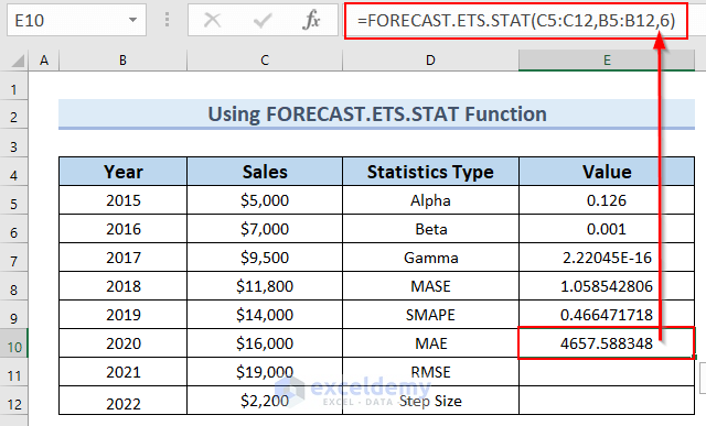
- To calculate the MAE value, enter the following formula in cell E10.
=FORECAST.ETS.STAT(C5:C12, B5:B12,6)
- Press ENTER.
- You can see the result in cell E10.
- To find the RMSE value, enter the following formula in cell E11.
=FORECAST.ETS.STAT(C5:C12, B5:B12,7)- Press ENTER.
- You can see the result in cell E11.
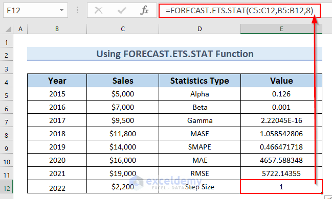
- To determine the Step Size value, enter the following formula in cell E12.
=FORECAST.ETS.STAT(C5:C12, B5:B12,8)
- Press ENTER.
- You can see the result in cell E12.
- The Value column is complete.
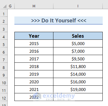
Practice Section
You can download the above Excel file and practice the explained methods.
Download Practice Workbook
You can download the practice workbook from here:
Related Articles
<< Go Back to Excel FORECAST Function | Excel Functions | Learn Excel
Get FREE Advanced Excel Exercises with Solutions!
