While collaborating with others on a worksheet, the updates are auto-saved. Changing in one section automatically changes the other. This goes for views too. It feels a bit frustrating when you work within a portion of the spreadsheet and suddenly the view changes because someone working on a different portion. Luckily, Microsoft Excel’s Sheet View is a wonderful solution for that. This tutorial will show you how to create different views for different users in Excel.
How to Create Different Views for Different Users in Excel: Step-by-Step Procedure
To create different views for different users in Microsoft Excel, we are going to use the Sheet View feature in Excel. A detailed description for each process is given below so that people with all ranges of knowledge in Excel can understand the process. We are going to create different views of the following dataset that is in the same Excel spreadsheet but for different users.

Follow these steps to see how we can accomplish that.
Step 1: Upload Workbook to OneDrive
If you go to the Sheet View group from the View tab, you will find that the options are grayed out.
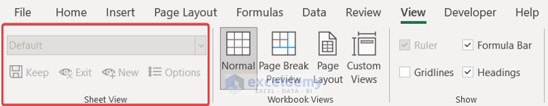
In order to resolve this problem first, you need to share or upload the workbook. As we may share this with different users at different points, sharing it on OneDrive could be the better option. You can directly share now with a particular use at this point if you wish.
- To upload it to OneDrive, click on the file name with a downward arrow beside it on top of the Excel workbook.
- Then click on Upload.
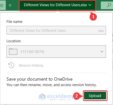
- Next, select the location and it will automatically upload the file to OneDrive.
Step 2: Create New Sheet View
Once you have uploaded the file, the Sheet View options will be available. To create a new view, go to the View tab on your ribbon. Then select New from the Sheet View group.

Step 3: Name Newly Created View
The next logical step would be to name the view. It will make the different views easier to find later on. You can name the view from the same Sheet View group under the View tab. Just click on the field above the Sheet View options and you can name your view there.
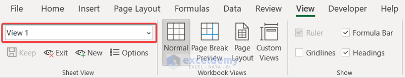
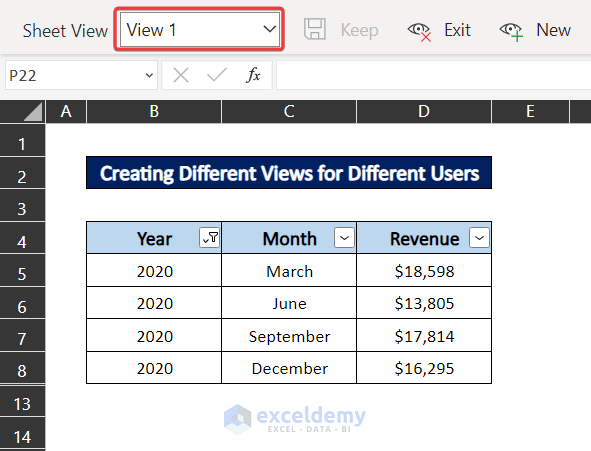
We named the first view “View 1” as shown in the figure.
Step 4: Make Modifications to Spreadsheet
Now it’s time to make the edits that can cause different views. We are choosing to use filter options for the demonstration here. You can also do your modifications in this step.
To add a filter to the dataset in the Excel spreadsheet, go to the Data tab on your ribbon. Then select Filter from the Sort & Filter group.

This will now create filter buttons in the column headings of the dataset.

Now let’s select data that only belongs to the year 2020 in the dataset for the first view. You can do that by clicking on the filter button in cell B4 and only checking 2020 from the drop-down menu. And then clicking on OK.

The dataset will now look like this.

This is going to be our first view.
Step 5: Share View with User
To share the view with a user, click on the Share option on the top-right of the ribbon.
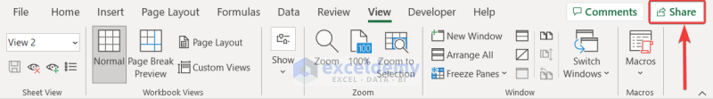
Then you can copy the link from there, or simply send the link through the mail.

The user going through the link will find this view and work with it in the browser.
Step 6: Repeat for All Users
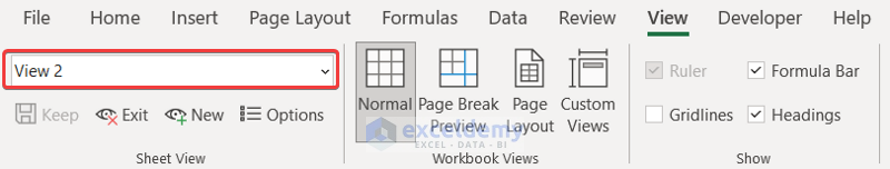
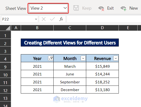
You can repeat all the steps for new views for different users. For example, let’s create another view called “View 2” as shown in steps 2 and 3.
And filter only data that belong to the year 2021.

Now sharing and opening the link will show us this view in the browser.
Repeat the process for all of the different views for different users in the Excel spreadsheet.
Read More: How to View All Sheets in Excel at Once
How to Filter in Excel Without Affecting Other Users
One of the major problems everyone complains about is filtering in one view would change the filtered view on others’ sheets too. As all of the shared people would share the exact copy, this was an obvious occurrence.
One apparent way to eliminate the problem is to create different views for different users either in Excel or from the browser. That is what the article was about after all. If each person has different views while working with the same worksheet, changing one’s filter’s values won’t change others too.
But let’s say you want to share the same sheets view with others. At the same time, you want to filter in the Excel spreadsheet without affecting other users. Luckily, Excel now has a feature that can help us filter only for us.
When you will use a filter in the dataset, Excel will warn you about how others are also using it and it will affect the users.
For example, let’s change the filter in cell B4 to this.

After clicking on OK, a warning box will appear as shown in the figure below. In the warning box, just select See just mine. This will filter in your Excel spreadsheet without affecting other users.

But it is still advisable to use different views for different users as all edits may not show this warning box.
Download Practice Workbook
You can download the workbook used for the demonstration from the download link below.
Conclusion
These were the procedure to create different views for different users in Excel and a solution for a common problem occurring while using the feature. Hopefully, you can easily make different views now. I hope you found this guide helpful and informative. If you have any questions or suggestions, let us know in the comments below.
Related Articles
<< Go Back to View in Excel | Learn Excel
Get FREE Advanced Excel Exercises with Solutions!
