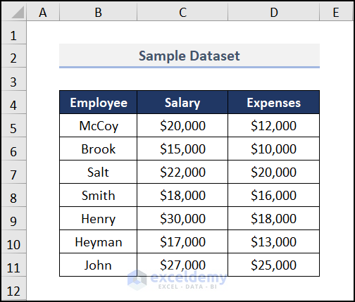
The sample dataset showcases Employees’ Salaries and Expenses.
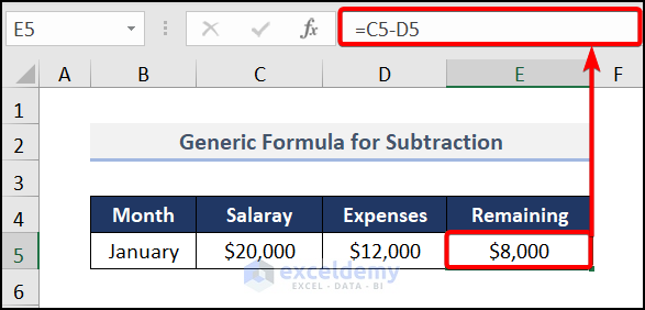
Method 1 – Subtraction Between Two Cells Using Generic Formula
Steps:
- Enter the formula in E5.
It subtracts D5 from C5.
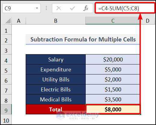
Method 2 – Using a Subtraction Formula with Multiple Cells
Steps:
- Enter the formula in C9.
The SUM(C5:C8) syntax adds the expenses from C5 to C8 and subtracts them from C4.
Read More: How to Subtract Multiple Cells in Excel
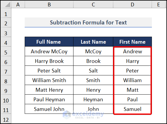
Method 3 – Using a Subtraction Formula for Text
To subtract the first name from the full name:
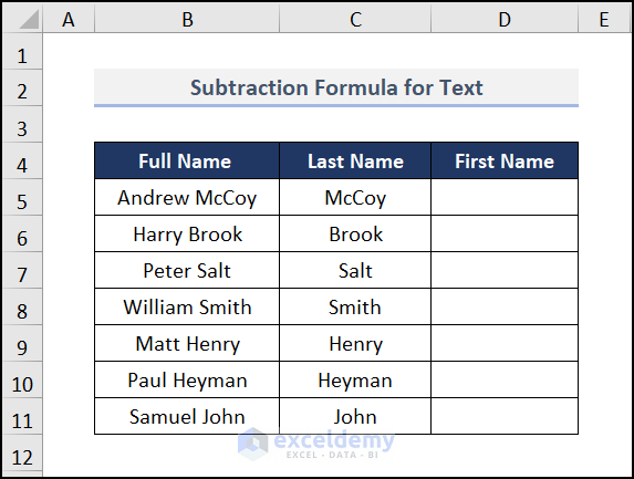
Steps:
- Enter the formula in D5.
Formula Breakdown:
SUBSTITUTE(B5, C5,””)→ takes the value of B5 and replaces the value in C5 with B5.
TRIM(SUBSTITUTE(B5, C5,””))→ takes the result of the SUBSTITUTE function and returns the value.
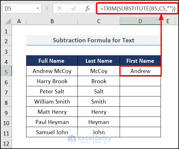
- Press ENTER to see the result.
Read More: How to Subtract in Excel Based on Criteria
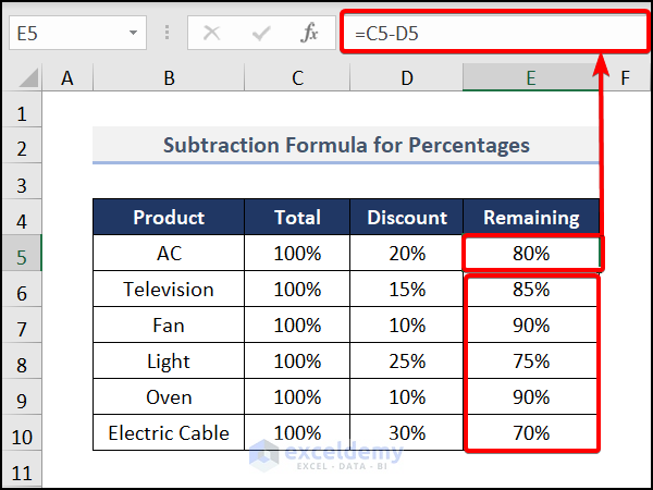
Method 4 – Using a Subtraction Formula for a Percentage
Steps:
- Enter the formula in E5.
The above formula subtracts the value of D5 from C5 and shows the result in percentage.
Read More: Excel formula to find the difference between two numbers
Method 5 – Using a Subtraction Formula Between Two Columns
Steps:
- Enter the formula in E5.
- Press ENTER to see the result.
- Drag down the Fill Handle to see the result in the rest of the cells.
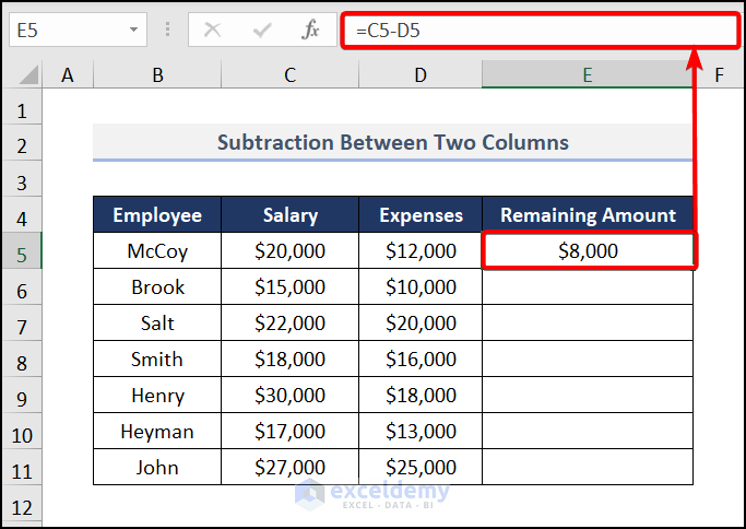
This is the output.
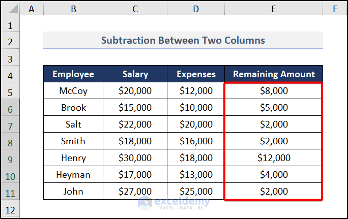
Read More: How to Subtract Two Columns in Excel
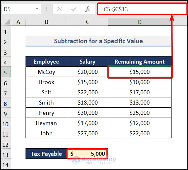
Method 6 – Using a Subtraction formula for a Specific Value Using Cell Reference
Steps:
- Enter the formula in D5.
$C$13 indicates the cell reference. Subtract the value of C13 from C5:C11 in this formula.
Read More: How to Subtract from Different Sheets in Excel
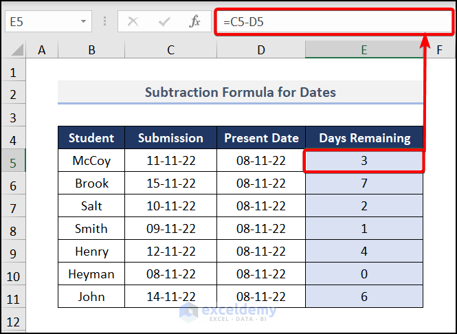
Method 7 – Using a Subtraction Formula for Dates
Steps:
- Enter the formula in E5.
It shows the remaining days counted from the entered date.
Read More: Excel VBA: Subtract One Range from Another
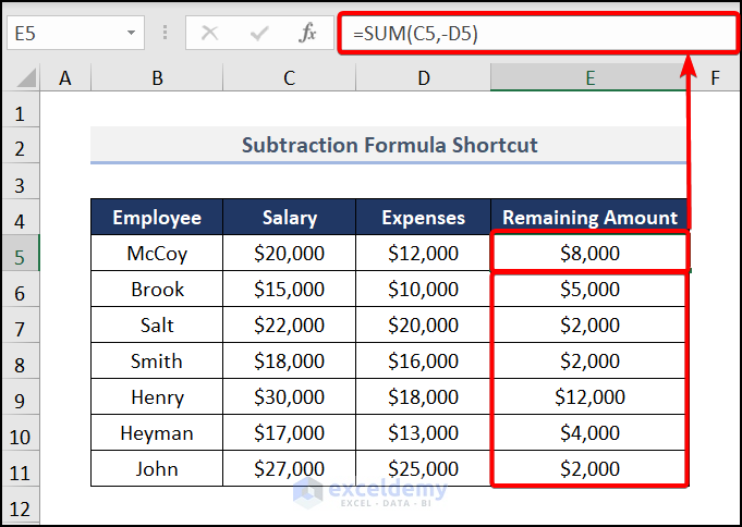
Using a Shortcut to Create a Subtraction Formula in Excel
- Enter the formula in E5.
The SUM function adds the value of these two cells, and the negative sign in the D5 makes all values in column D negative.
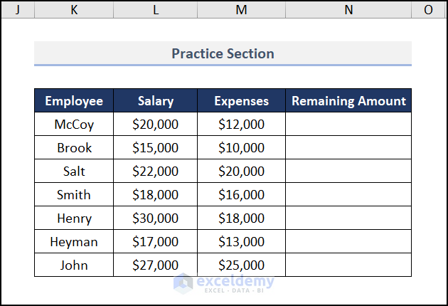
Practice Section
Practice here.
Download the following practice workbook.
Related Articles
<< Go Back to Subtract in Excel | Calculate in Excel | Learn Excel
Get FREE Advanced Excel Exercises with Solutions!
