Subtraction definition and nomenclature
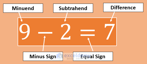
- Minuend: A quantity or number from which another is to be subtracted. In the above example, 9 is the minuend.
- Minus Sign (-): Then we use a minus symbol (-) to find the difference between two numbers.
- Subtrahend: Subtrahend is the quantity or number to be subtracted from minuend.
- Equal Sign (=): Then we place an equal sign (=).
- Difference: Difference is the result of the subtract operation.
How to Find the Difference Between Two Numbers Using Excel Formula
Method 1 – Using Numbers Directly in the Formula
- Input an equal sign (=) to start an Excel formula
- Input the minuend value.
- Input the minus sign (-).
- Place the subtrahend value.
- Press Enter.
Example: =50-5
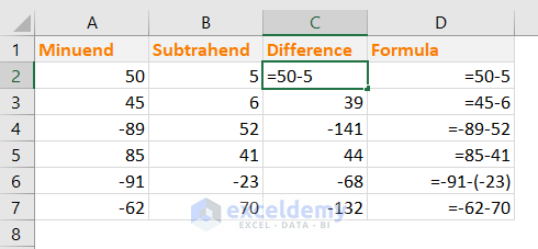
Note: If the subtrahend value is negative, use the parentheses to place the number in the subtraction formula like this: =-91-(-23)
Why is this method not suggested?
- If you have more than one subtraction, you have to write a formula for every subtraction individually
- You cannot copy the same formula for another set of numbers
- Time-consuming as you have to write a formula for every set of numbers individually
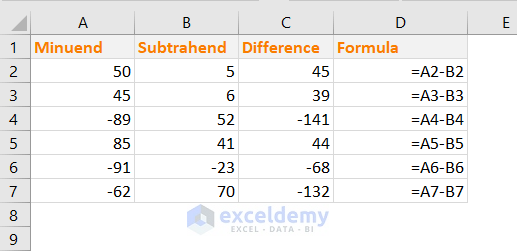
Method 2 – Using Cell References Instead of Numbers in the Formula
- In the cell C2, input this formula: =A2-B2
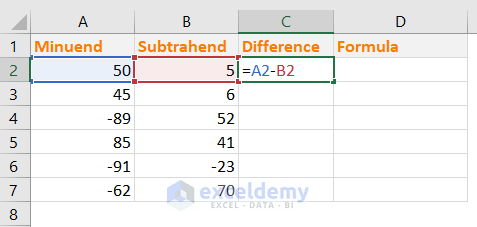
- Press Enter.
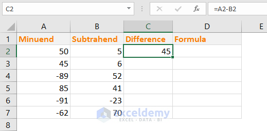
- Copy this formula for other cells in the column. You can apply the same formula to multiple cells in Excel in more than one way.
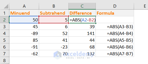
Method 3 – Calculate the Absolute Difference Between Two Numbers in Excel with the ABS Function
The ABS(number) function returns the absolute value of a number, i.e., without its sign.
Here’s an example of using the formula to get the absolute differences.
Read More: How to Subtract Two Columns in Excel
The Percentage Difference Between Two Numbers in Excel
Here’s the equation to calculate the Percent Difference.

E1 = First experimental value and E2 = Second experimental value
- Use this formula in cell C2: =2*ABS(A2-B2)/(A2+B2)
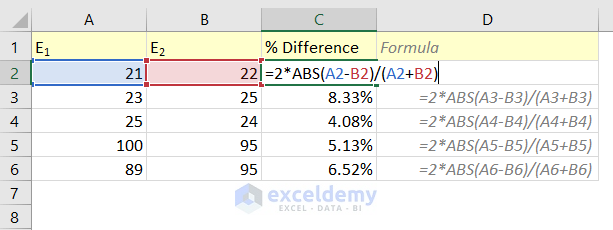
How does this formula work?
- The difference between numbers A2 and B2 (A2-B2) can be negative. We have used the ABS() function (ABS(A2-B2)) to make the number absolute.
- We multiplied the absolute value by 2, then divided the value by (A2+B2)
Read More: How to Create a Subtraction Formula in Excel
Calculate the Percentage Change for Negative Numbers in Excel
Theoretically and even practically, you cannot find the percentage change for negative numbers. When it is not possible theoretically, how can we calculate them in Excel?
Not possible. Whatever methods you use, you will find misleading results.
Here I will show 3 methods to calculate the percentage change of negative numbers in Excel but all of them will mislead you. So, be aware of it before using them in your work.
Method 1 – Calculate the % change of Negative Numbers by Making the Denominator Absolute
We want to calculate the percentage of two values:
Old value: -400
New value: 200
We’ll use the formula: % change = ((New value – Old value)/ Old value) x 100%
If we apply this formula to calculate the % change of the two above values (-400 & 200), this will be the result:
= ((200 – (-400))/-400)*100%
= 600/(-400)*100%
= -150%
This is a completely wrong answer.
Some companies use the ABS method. In this method, the denominator is made absolute.
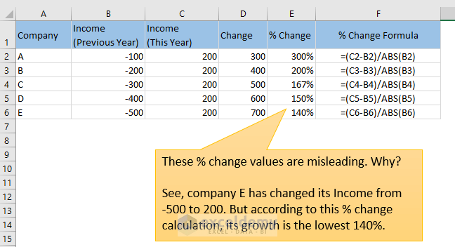
These results are also misleading because you see -100 to 200 shows the biggest % change when -500 to 200 shows the smallest % change.
Take a look at the following image:
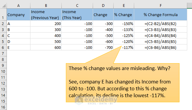
These results are also misleading.
You see, though company E has seen the sharpest decline in income (from 600 to -100), the % change is showing that it has declined the lowest (-117%).
Method 2 – Shift the Numbers to Make Them Positive
We have two values:
Old value: -50
New value: 20
We will shift these two numbers using their absolute values and then multiplying by 2: (|-50|+ |20|)*2 = 140
shifted_old value = -50 + 140 = 90
shifted_new value = 20 + 140 = 160
The resulting % change: ((160-90)/90)*100% = 77.78%
Let’s see whether this method gives us satisfactory results:
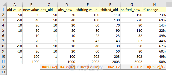
The last row shows a stark difference in the expected result.
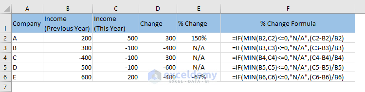
Solution: Show N/A (or anything) When the % Change of Negative Numbers Appears
Here’s the general formula:
<code>IF(MIN(old_value, new_value)<=0, “N/A”, (new_value-old_value)/old_value)
Download the Excel File
Related Articles
- Subtraction for Whole Column in Excel
- How to Subtract from Different Sheets in Excel
- Excel VBA: Subtract One Range from Another
- How to Subtract in Excel Based on Criteria
- How to Subtract from a Total in Excel
- How to Subtract Multiple Cells in Excel
<< Go Back to Subtract in Excel | Calculate in Excel | Learn Excel
Get FREE Advanced Excel Exercises with Solutions!

But what if it’s time what you’re calculating??
Dear DON_1234567,
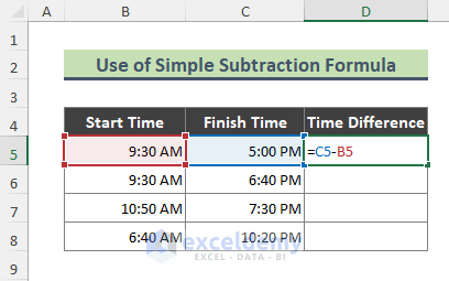
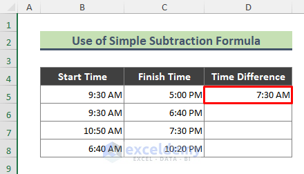
You can use the simple subtraction formula to calculate the difference between two times.
You can use the formula below-
=C5-D5Check out the screenshot below-
If you are still not getting the result. Then change the cell format to time.
You can visit the below article to learn more. Thanks!
Calculate Difference Between Two Times
Thanks, Kawser! You ABSolutely save me! Is there a list showing common formulas somewhere? I takes so long to come up with them on my own.
Can you please help me with counting the number of the total from opening and closing?
For example
My opening number is 6
My closing number is 12
Then the total number should be 7(including opening number) rather than 6.
Can you please help me with counting the number of the total from opening and closing?
For example
My opening number is 6
My closing number is 12
Then the total number should be 7(including opening number) rather than 6.
Dear KOLAPALLI PAVAN KUMAR,
The output you are looking for can be achieved using the COUNT function in excel. Here the COUNT function counts the cell number given in the string.
Apply the following formula-
=COUNT(C2:C8)You can check the screenshot below-
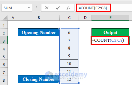
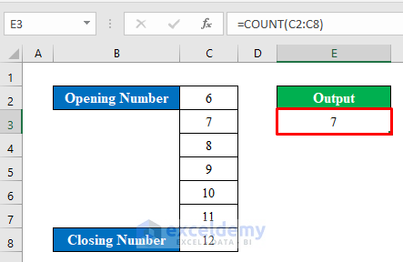
First, select a cell (E3) to apply the formula.
Second, press Enter to get the desired output.
Hope you got your solution. If you still didn’t get it, check out the article below-
The Different Ways of Counting
Thanks!
Solution:
=ABS(ABS(Q34-R34)/(Q34+R34))*(IF(Q34>R34;-1;1))
=ABS(ABS(Q34-R34)/(Q34+R34))*(IF(Q34>R34;-1;1))
hi
I need one formula for Excel
there are three numbers for the same digit another number and two numbers same
output result required
how many numbers are more than two
example
2210001
2210001
2210002
2210002
2210003
2210003
2210003
2210004
2210006
2210006
2210006
2210006
2210007
2210007
2210009
2210009
2210009
Hi ISRAVEL,
To achieve this in Excel, you can use the COUNTIF function to count the occurrences of each number and then check which numbers occur more than twice. Here’s how you can set up your Excel sheet:
Assuming your numbers are in column A starting from A2, you can use the following formula in another cell to get the count of numbers that appear more than twice:
=COUNTIF(A:A, A2)Drag down this formula for each number in your list. This will give you the count of each number.
Then, you can use another column to check if the count is greater than 2:
=IF(B2>2, "More than two", "Not more than two")Drag this formula down for each number in your list.
This setup will give you a clear indication of which numbers occur more than twice in your list.
I hope this comment will help you get your required output. Please let us know in the comment section if you have any other queries.
Regards
Maruf Hasan
ExcelDemy