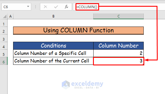
Example 1 – Using COLUMN Function
In the given sample dataset, we will use the COLUMN function for two conditions. The first condition is for finding out the column number of a specific cell and the second one is for the current working cell.
Step 1:
- To find out the column number of a specific cell, use the following formula of the COLUMN function mentioning the cell. We will use cell B5.
=COLUMN(B5)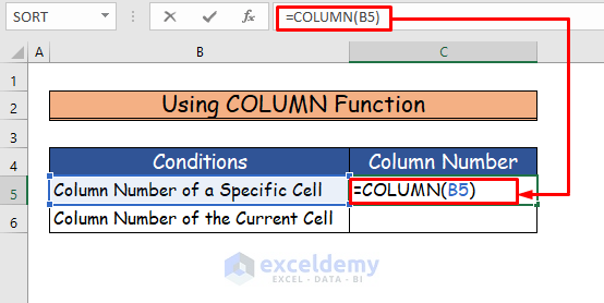
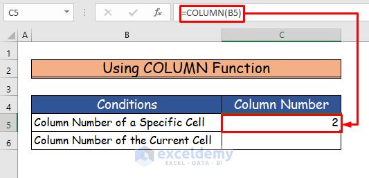
- After pressing Enter, you will see the column number of the mentioned cell, which is column number 2 for cell B5.
Step 2:
- To determine the column number of the current cell on which you are working, use the following formula of the COLUMN function.
=COLUMN()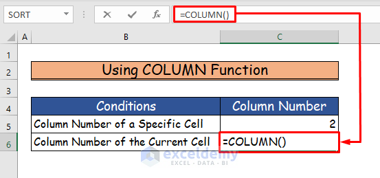
- After pressing Enter, you will see the column number of the current working cell, which is number 3 for cell C6.
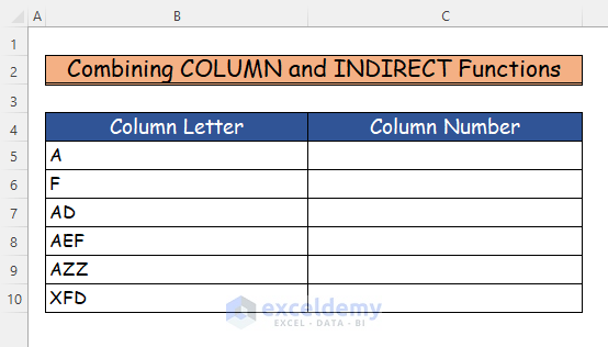
Example 2 – Combining COLUMN and INDIRECT Functions
We will select some column headers of an Excel worksheet randomly in column B and find out their column numbers in column C.
Step 1:
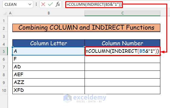
- Enter the following formula in cell C5, which is the combination of the COLUMN function and the INDIRECT function.
=COLUMN(INDIRECT(B5&"1"))- We will input this formula in cell C5 to determine the column number of column A which is in cell B5.
Step 2:
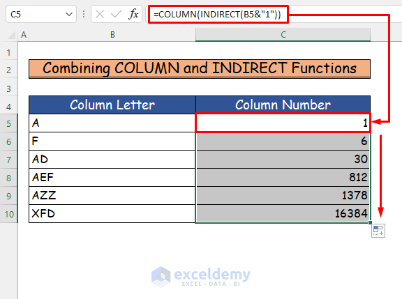
- Press Enter and you will see the column number of column A in cell C5 which is 1.
- Use AutoFill to drag down the formula to the remaining cells.
- You will see all the column numbers in their respective cells.
- INDIRECT(“B5”) will take the cell value of B5 which is A.
- INDIRECT(B5&1) receives the previous output and connects 1 to the previous code’s output to make it A1.
- COLUMN(INDIRECT(B5&”1″)) will show the column number of cell A1, which is 1.
Read More: How to Change Column Name from ABC to 1 2 3 in Excel
Example 3 – Applying Non-Volatile Formula
If you are working with a large dataset, you can use the MATCH function and the ADDRESS function with the COLUMN function as they are both volatile.
Step 1:
- Enter the following formula in cell C5.
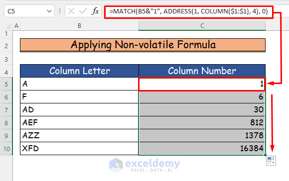
=MATCH(B5&"1", ADDRESS(1, COLUMN($1:$1), 4), 0)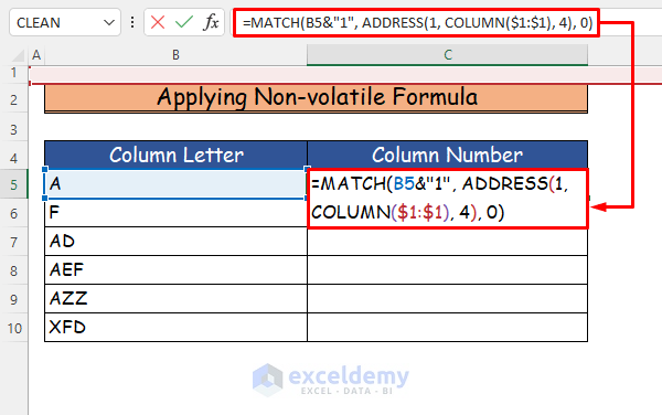
Step 2:
- Press Enter and you will see the column number of the column.
- Use the Autofill Handle tool for the remaining cells.
- COLUMN($1:$1) represents all the columns of the first row in the worksheet.
- ADDRESS(1, COLUMN($1:$1), 4) will make an arrangement of texts with the first row and all the columns of the worksheet. For example, “A1”, “B1” etc. until the worksheet ends.
- The formula MATCH(B5&”1″, ADDRESS(1, COLUMN($1:$1), 4), 0) matches the cell value given in cell B5 converted into cell reference, which is A1 and returns where it matches in the previous arrangement.
- 0 is given to find an exact match in the formula.
Read More: How to Convert Column Number to Letter in Excel
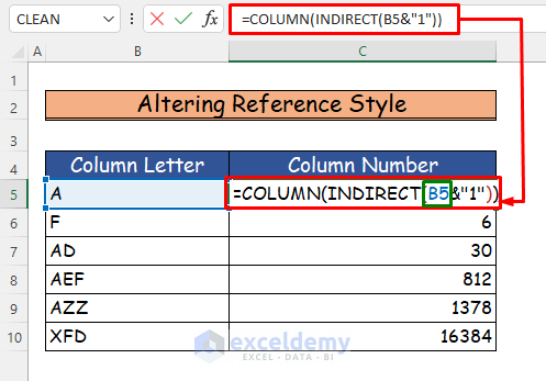
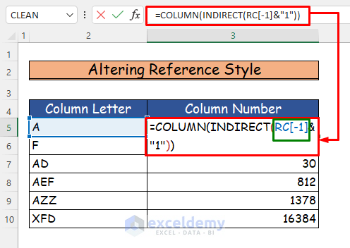
Example 4 – Altering Reference Style
The reference in the formula of cell C5 shows the cell number in column letter which is B5. We will convert the column letter to number by altering the reference cycle.
Step 1:
- Go to the File tab on the ribbon.
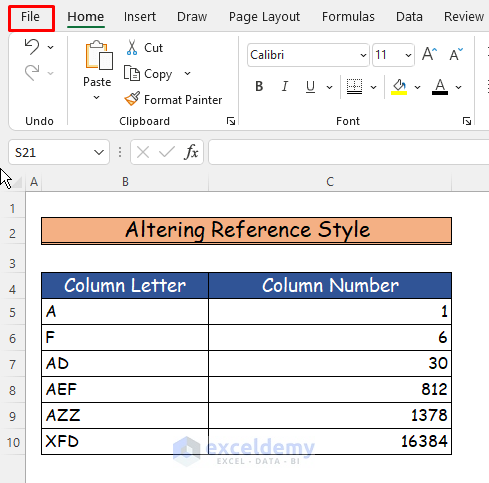
- Select the Options command.

Step 2:
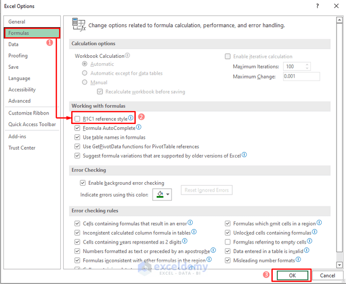
- After choosing the command, you will find a dialog box, Excel Options.
- From the Formulas tab, mark the option named R1C1 reference style.
- Click OK.
Step 3:
- You will see that your worksheet will have the R1C1 reference style, in which the columns of the worksheet will be transformed into numeric values.
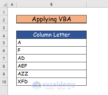
Example 5 – Applying VBA to Convert Column Letter to Number in Excel
We will use the following data set to apply VBA.
Step 1:
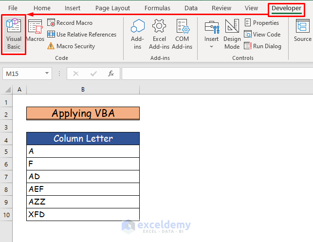
- Choose the Visual Basic command from the Code group in the Developer tab.
Step 2:
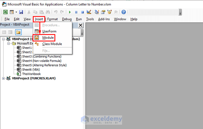
- Choose the Module command in the Insert tab.
Step 3:
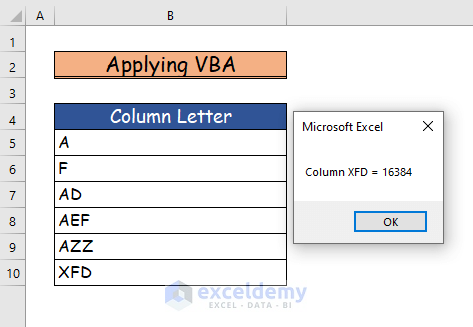
- Enter the following VBA Code into the Module. We will insert the column letter XFD to find out its column number.
Sub Excel_Column_Letter_to_Number_Converter()
'Convert a specific Column Letter into it's corresponding Numeric Reference
Dim ColumnNumber As Long
Dim ColumnLetter As String
'Call the Column Letter
ColumnLetter = "XFD"
'Convert To the Column Number
ColumnNumber = Range(ColumnLetter & 1).Column
'Show the Final Result
MsgBox "Column " & ColumnLetter & " = " & ColumnNumber
End Sub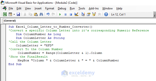
- Save the code and press the play button to activate it.

Step 4:
- After running the code, you will see the corresponding column number of XFD which is 16384.
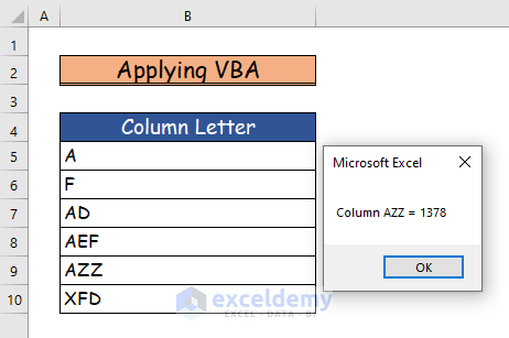
- You can run this code for other column letters as well and find their respective column number.
Read More: Find Value in Row and Return Column Number Using VBA in Excel
Download Practice Workbook
Related Articles
- How to Return Column Number of Match in Excel
- How to Find Column Number Based on Value in Excel
- How to Find Column Index Number in Excel
- VBA to Convert Column Number to Letter in Excel
- How to Use VBA Range Based on Column Number in Excel
<< Go Back to Learn Excel
Get FREE Advanced Excel Exercises with Solutions!
