How to Change Column Name from ABC to 1 2 3 in Excel

Method 1 – Use the R1C1 Reference Style to Change Column Names

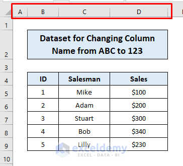
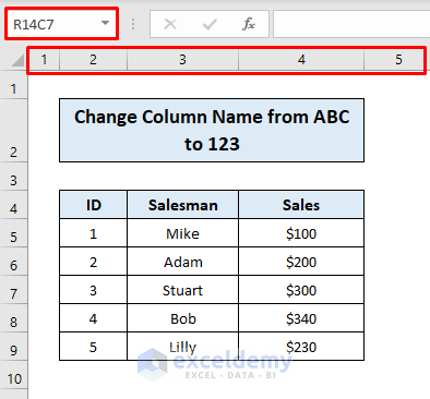
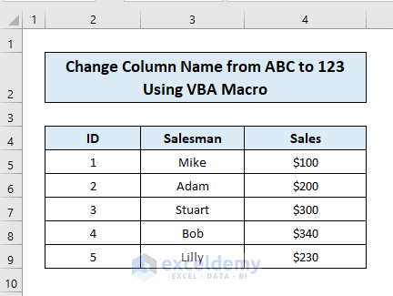
We have a dataset of sales of the sales assistants of a shop over a certain period of time. However, the contents of the dataset don’t particularly matter.

Go to the File tab on the ribbon.

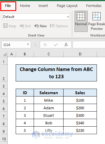
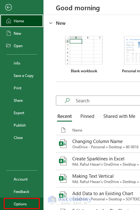
Click Options from the menu list (you may need to go to More).

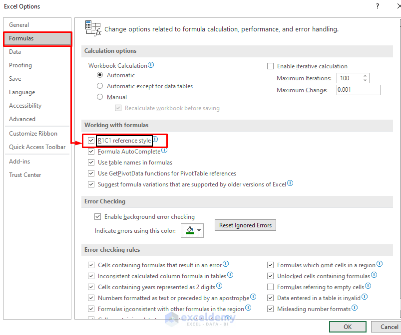
Go to the Formulas section.
Check R1C1 reference style.
Press OK.

Excel has changed the column headings from an alphabetical to a numerical order. The reference style will show up in the left corner.

Method 2 – Using VBA Macro to Change Excel Column Names

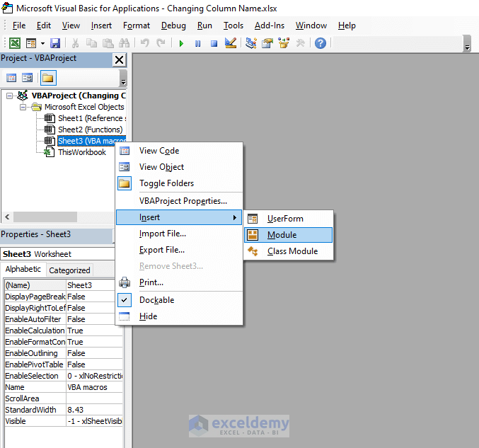
Open a new worksheet and press Alt + F11.
The Visual Basic Editor window will show up.
Right-click on the workbook name (i.e. Sheet 3) from the file manager on the left.
Choose Insert and click Module from the options.

Copy this VBA code and paste it into the module:

Sub ColumnNames123()

    Application.ReferenceStyle = xlR1C1

End Sub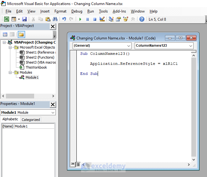

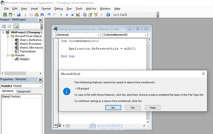
Save the file as an “Excel Macro-enabled Workbook” and press Alt + Q to close this window.

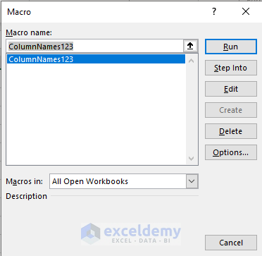
Press Alt + F8 and a Macro dialog box will pop up.
Select ColumnNames123 from the Macro name box and click on Run.

This applies the R1C1 reference style, changing the column header names.

By following this way, you can change the column headings of your Excel workbook from A B C to 1 2 3.

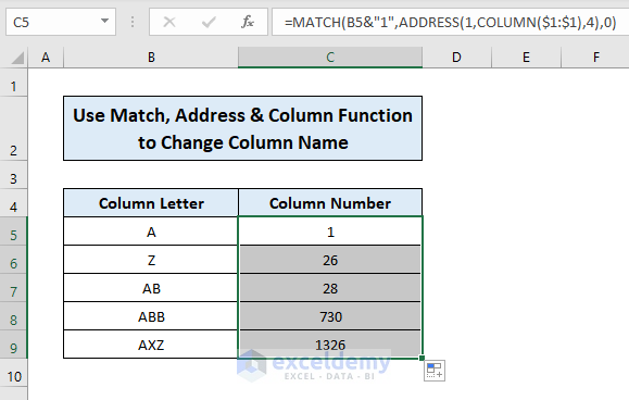
Alternative Method to Change Column Name to 123 in Cells

Use the following formula in the cell C5:

=MATCH(B5&"1",ADDRESS(1,COLUMN($1:$1),4),0)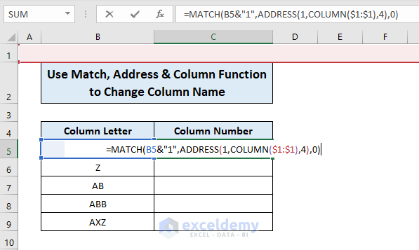

Formula Breakdown

»ADDRESS(1,COLUMN($1:$1),4)

1= Row number
COLUMN($1:$1)= Sequence of column numbers
4= Relative reference

So, the ADDRESS function returns this array:

{“A1”, “B1”, “C1”, “D1”,….., “XFD1”}

»MATCH(B5&”1”,{“A1”, “B1”, “C1”, “D1”,….. “XFD1”},0)

B5= A (Value of Cell B5)
1= Row number

The string becomes A1

»MATCH(A1,{“A1”, “B1”, “C1”, “D1”,….. “XFD1”},0)

The MATCH function searches the string A1 in the above array and returns the position of the found value (column number).

Press Enter and you will get the corresponding column number.

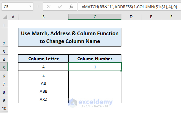
Use Autofill to drag the formula to the rest of the cells and you will get the output.

Download the Practice Workbook

Changing Column Name.xlsm

<< Go Back to Column Number | Columns in Excel | Learn Excel

Get FREE Advanced Excel Exercises with Solutions!

How to Change Column Name from ABC to 1 2 3 in Excel

Method 1 – Use the R1C1 Reference Style to Change Column Names

Method 2 – Using VBA Macro to Change Excel Column Names

Alternative Method to Change Column Name to 123 in Cells

Related Articles

Leave a reply Cancel reply