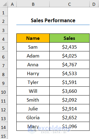
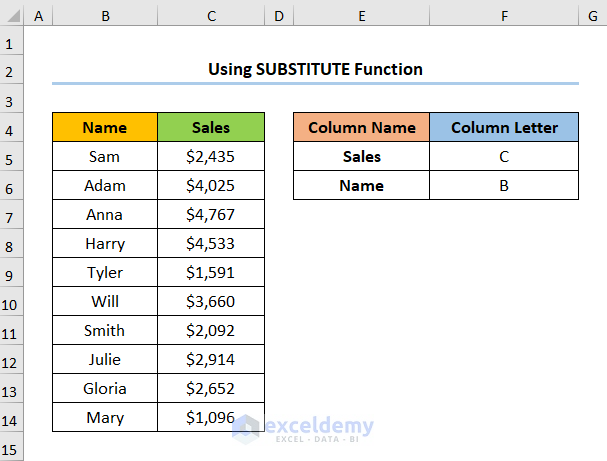
Consider the following dataset.
Method 1 – Using the MATCH Function to Return Column Number of Match
Steps:
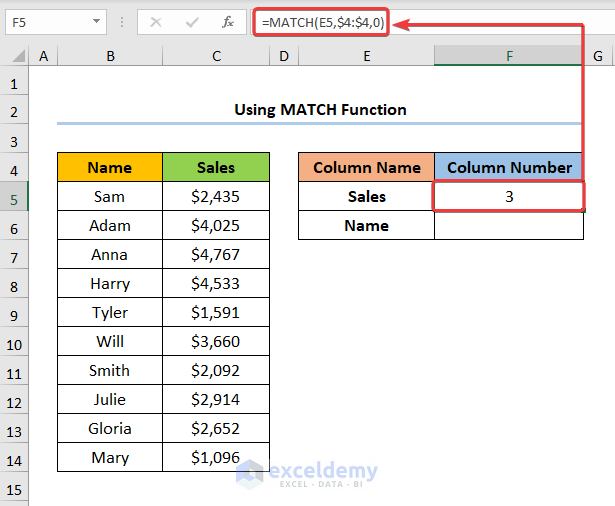
- Enter this formula in F5.
=MATCH(E5,$4:$4,0)
E5 cell refers to the Sales, and $4:$4 indicates Row Number 4; 0 (match_type argument) represents the Exact match criteria.
Note: Provide an Absolute Cell Reference for the first C5 by pressing F4.
- Drag down the Fill Handle Tool to copy the formula.
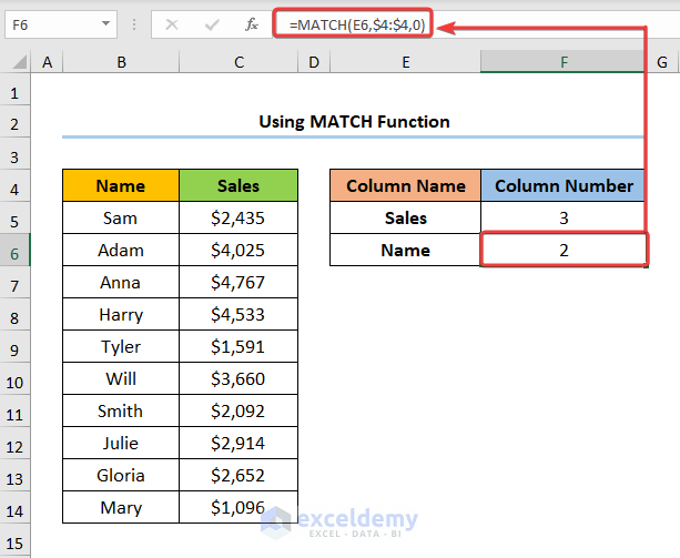
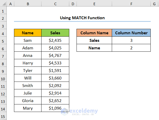
This is the output.
Read More: Column Letter to Number Converter in Excel
Method 2 – Return a Matched Column Number with the COLUMN Function
Steps:
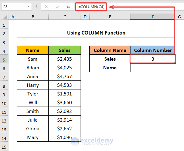
- Enter this formula in F5.
=COLUMN(C4)
The COLUMN function takes the reference argument and returns the column number of a reference cell. Here, C4 is the reference argument (Sales).
- Enter the COLUMN function and B4 as cell reference for the Name.
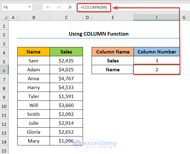
This is the output.

Read More: How to Change Column Name from ABC to 1 2 3 in Excel
Method 3 -Using the SUBSTITUTE Function to Obtain a Column Letter from a Specific Cell
Steps:
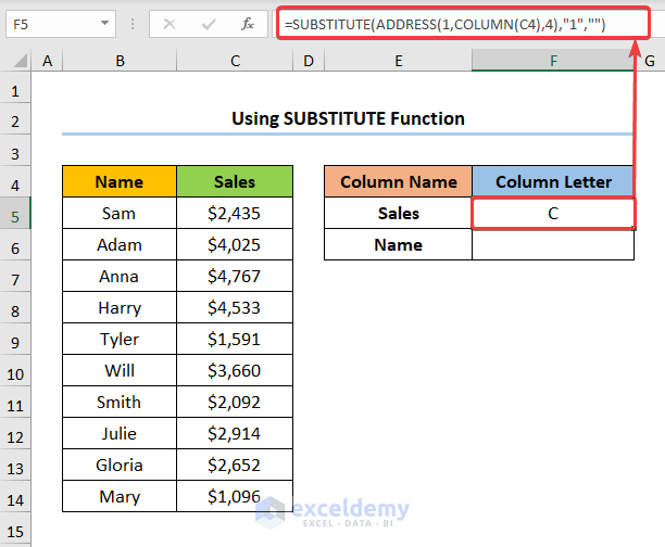
- Enter this formula in F5.
=SUBSTITUTE(ADDRESS(1,COLUMN(C4),4),"1","")
C4 refers to Sales.
Formula Breakdown:
- COLUMN(C4) → returns the column number of C4.
- Output → 3
- ADDRESS(1,COLUMN(C4),4) → becomes
- ADDRESS(1,3,4) → creates a cell reference as text. 1 is the row_number argument and 3 is the column_number argument. 4 represents the optional abs_num argument which contains the ADDRESS function to return a Relative Reference.
- Output → C1
- =SUBSTITUTE(ADDRESS(1,COLUMN(C4),4),”1″,””) → becomes
- =SUBSTITUTE(C1,”1″,””) → Replaces existing text with new text. Here, C1 refers to the text argument (Sales). “1” is the old_text argument, and the “” refers to the new_text argument which is left blank.
- Output → C
- Repeat the process for F6.
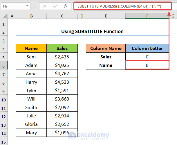
This is the output.
Method 4 – Applying a VBA Code to Return a Matched Column Number in Excel
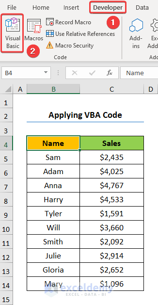
Step 1: Open Visual Basic Editor
- Go to the Developer tab >> click Visual Basic.
Visual Basic Editor will open in a new window.
Step 2: Use the VBA Code
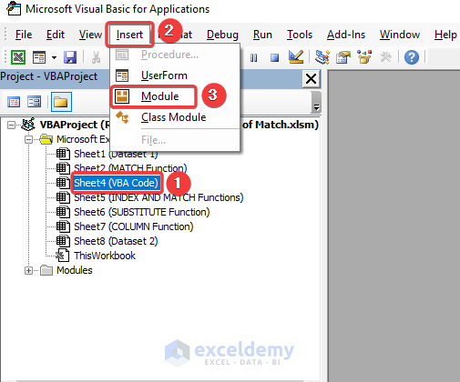
- Choose the Sheet to insert a Module. Here, Sheet4 (VBA Code).
- Go to the Insert tab >> select Module.
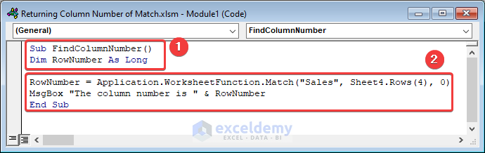
- Enter the following code.
Sub FindColumnNumber()
Dim RowNumber As Long
RowNumber = Application.WorksheetFunction.Match("Sales", Sheet1.Rows(3), 0)
MsgBox "The column number is " & RowNumber
End Sub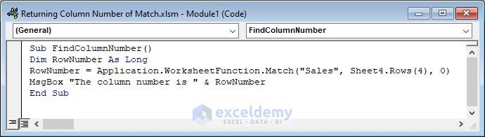
Code Breakdown:
- The sub-routine is given a name.
- The variable RowNumber is defined and the Long data type is selected.
- The MATCH function determines the Column Number of the Sales header.
- RowNumber stores this value.
- the MsgBox function displays the result.
Step 3: Run the VBA Code
- Press F5.
- In the Macros dialog box, click Run.
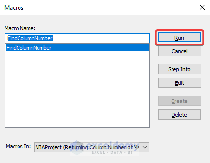
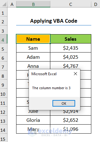
A window is displayed showing the Column Number.
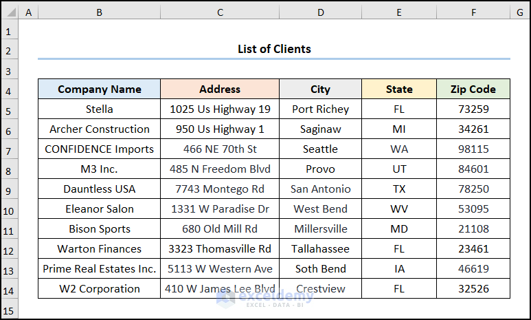
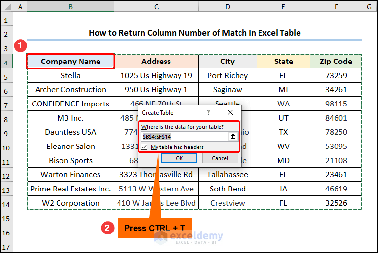
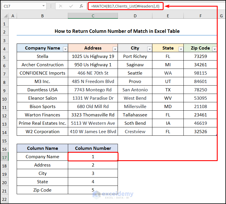
Method 5 – Utilizing an Excel Table to Return the Column Number of Match
This is the dataset.
Steps:
- In B4 >> press CTRL + T to insert an Excel Table.
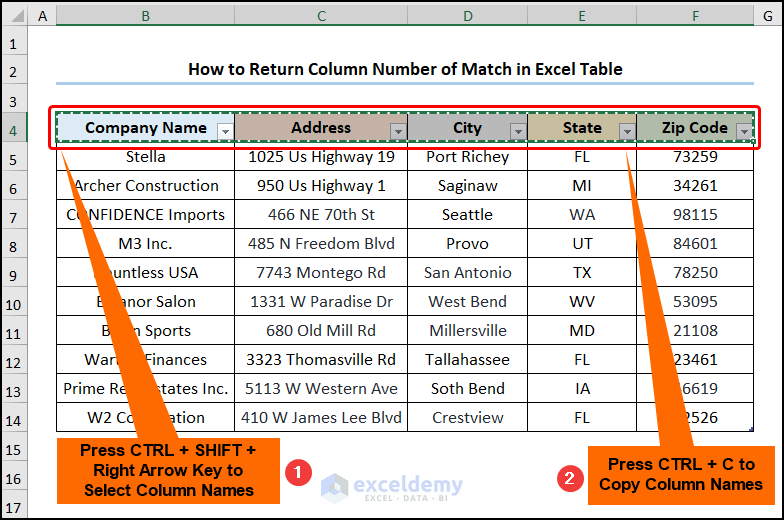
- Press CTRL + SHIFT + Right Arrow (->) to select all column headers >> Press CTRL + C to copy them.
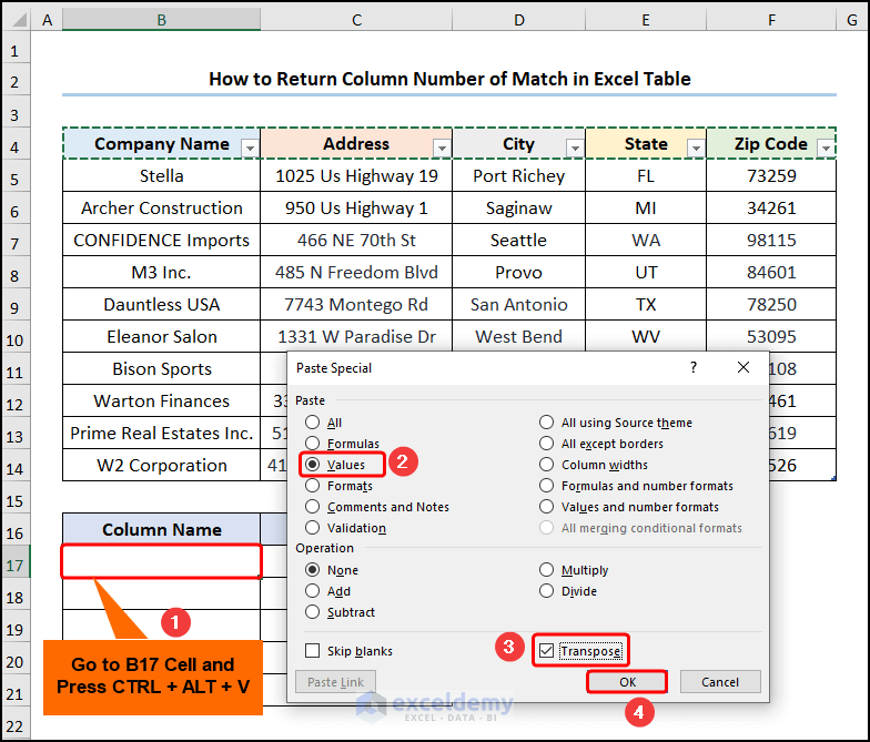
- Press CTRL + ALT+ V to open Paste Special >> check Values and Transpose >> Click OK.
This is the output.
- Enter this formula in C17 >> drag the Fill Handle tool to copy the formula.
=MATCH(B17,Clients_List[#Headers],0)
B17 refers to the Company Name whereas Clients_List is the name of the Excel Table.
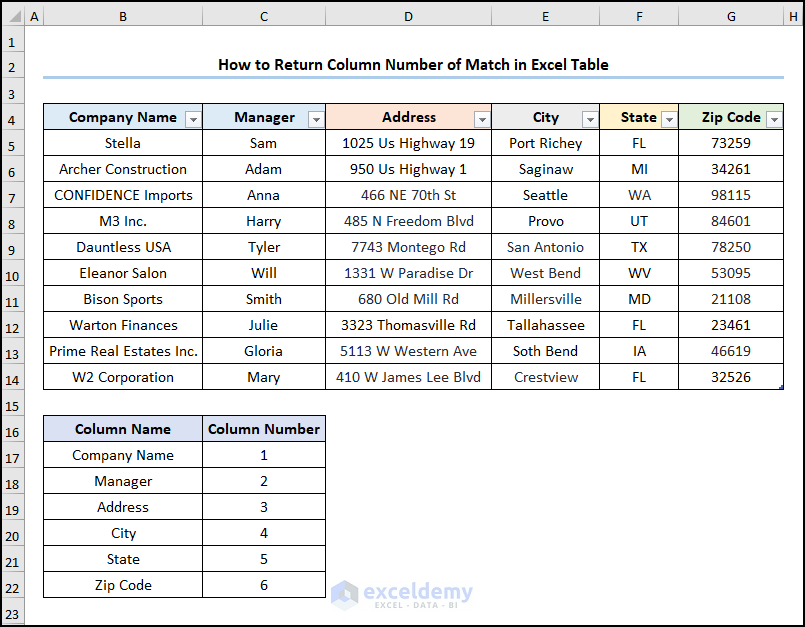
- Insert an extra Manager column and Column Numbers will change.
You can also find a specific value in rows and return the column number by using a VBA code.
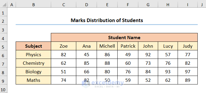
Return Value for a Match Column Using the INDEX and MATCH Functions
This is the sample dataset.
Steps:
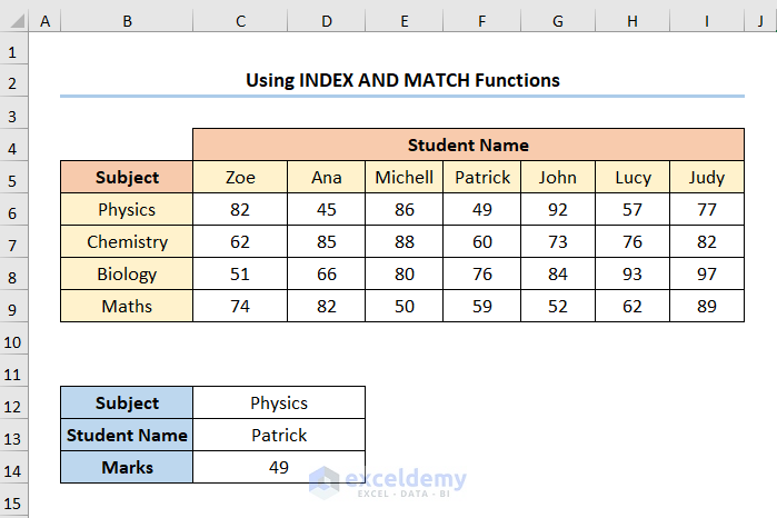
- Choose a Subject and enter the Student Name. Here, Physics and Patrick.
- Go to C14 and enter the formula below.
=INDEX(C6:I9,MATCH(C12,B6:B9,0),MATCH(C13,C5:I5,0))
Here, the C6:I9 range represents the marks scored by the students in the 4 Subjects.
Formula Breakdown
- MATCH(C12, B6:B9,0) → returns the relative position of an item in an array matching the given value. Here, C12 is the lookup_value argument (Physics). B6:B9 represents the lookup_array argument that searches the match. 0 is the optional match_type argument which indicates Exact match criteria.
- Output → 1
- MATCH(C13, C5:I5,0) → In this formula, C13 is the Student Name Patrick. C5:I5 is the array from which Patrick is matched. 0 indicates Exact match criteria.
- Output → 4
- =INDEX(C6:I9,MATCH(C12,B6:B9,0),MATCH(C13,C5:I5,0)) → becomes
- =INDEX(C6:I9,1,4) → Returns a value at the intersection of a row and column in a given range. In this expression, C6:I9 is the array argument (marks scored by the students). 1 is the row_num argument (the row location). 4 is the optional column_num argument (column location).
- Output → 49
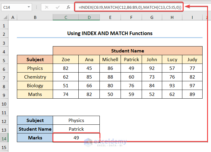
This is the output.
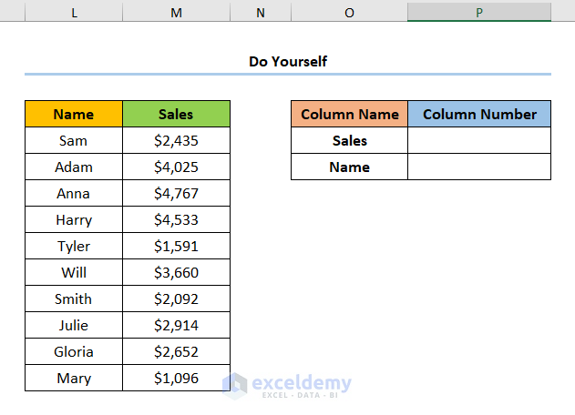
Practice Section
Practice with this sample dataset.
Download Practice Workbook
Related Articles
- How to Find Column Index Number in Excel
- How to Convert Column Number to Letter in Excel
- How to Find Column Number Based on Value in Excel
- VBA to Convert Column Number to Letter in Excel
- How to Use VBA Range Based on Column Number in Excel
<< Go Back to Learn Excel
Get FREE Advanced Excel Exercises with Solutions!
