In general, conditional formatting is now an integral part of the Microsoft Excel experience. This helps us identify particular values in a random or large group of data. Moreover, we can not only identify certain values but also identify which belong to a certain range or not in string values, numeric values, errors, etc., with conditional formatting. However, it is, as the name suggests, Excel formatting a cell based on whether a condition is true or not. In this tutorial, I will show you a step-by-step procedure on how to make a checklist with conditional formatting in Excel.
How to Make Checklist with Conditional Formatting in Excel: Step-by-Step Procedure
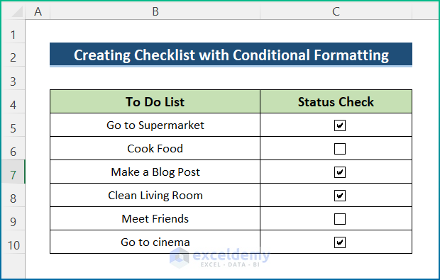
Fortunately, you can make a checklist with conditional formatting in Excel easily. This time, I will make a checklist beside a set of data. With the options checked, the original data will change its format. However, you have to follow the steps mentioned below in order to properly complete the operation. For example, I have selected some daily tasks which need to be completed.
Step 1: Select Dataset in Excel
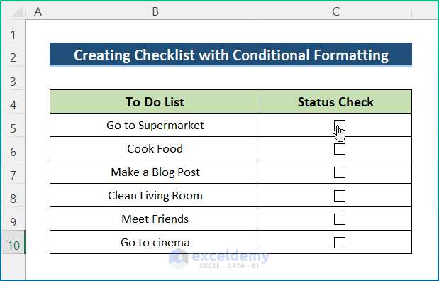
For the purpose of demonstration, I have used the following sample dataset.
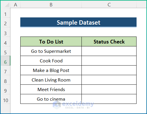
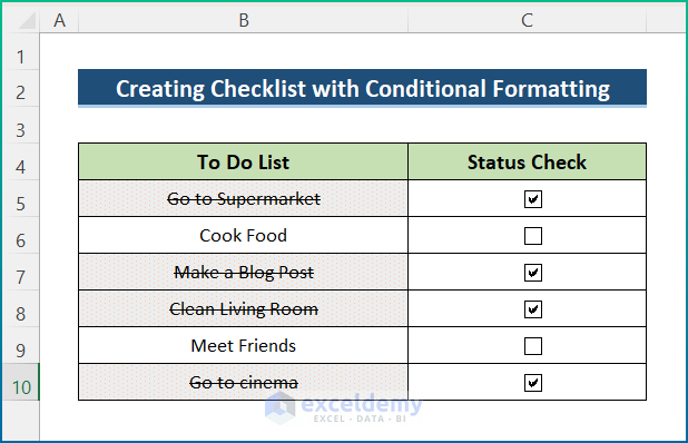
This is a standard to-do list. Once you check a checkbox in the status column, the task beside it will change the format, let’s say, a strikethrough. However, the basic idea is to use the boolean value of the checkbox to format in column B.
Step 2: Create Check Boxes
- First, go to the Developer tab on your ribbon.
- Then, select Insert from the Controls group section.
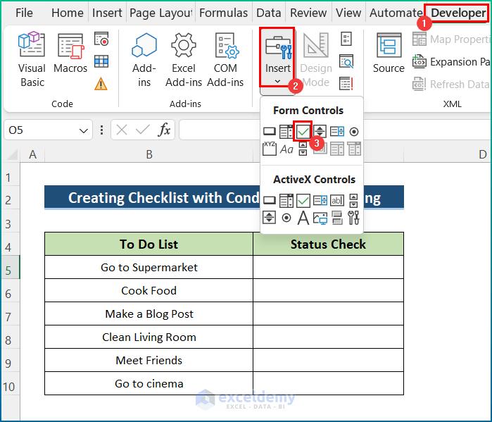
- Next, the cursor will look like a “+” sign, and drag your cursor while holding the left button of the mouse to create a check box.

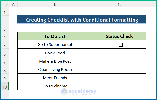
- Now, use the Backspace button to delete the text.
- After that, hold the left button of your mouse to move the check box to put it in the middle of the cell.
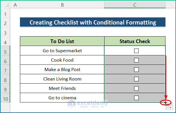
- Finally, utilize the AutoFill tool for the entire column.
Read More: How to Make a Checklist in Excel
Step 3: Mark Check Boxes
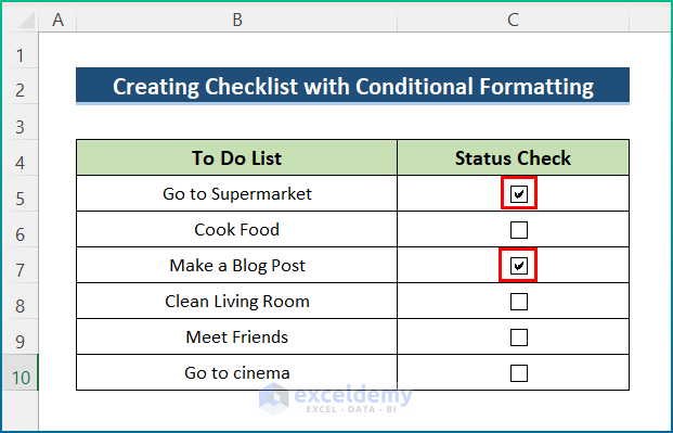
- First of all, move your cursor to the check box you want to check.
- However, once your cursor is near the box, the cursor will look like a Hand Icon.
- At last, you can click on the box to check the box.
Read More: How to Make a Daily Checklist in Excel
Step 4: Link Cells
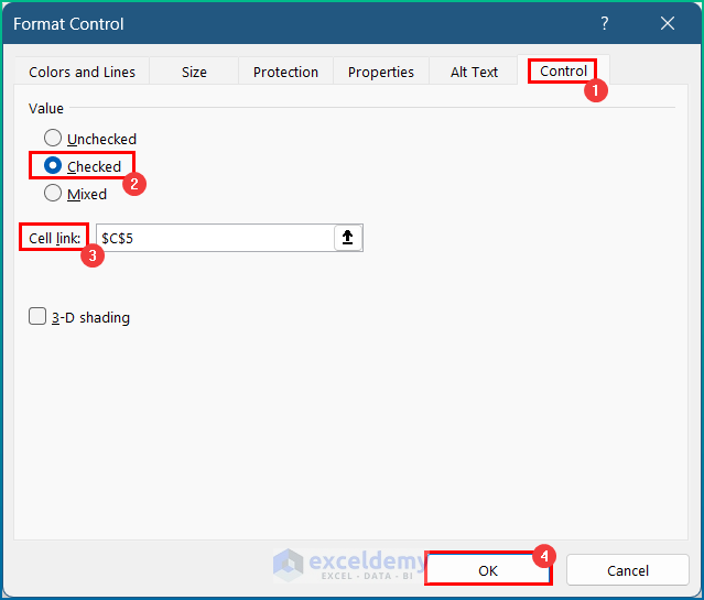
- Initially, right-click on the box and select Format Control from the context menu.

- Then, go to the Control tab on the box and select cell C5 as its linked cell.
- Next, select OK.
- Similarly, follow the process to each cell of the column.
- Once checked, there will be a TRUE/FALSE value on the cells, depending on it.
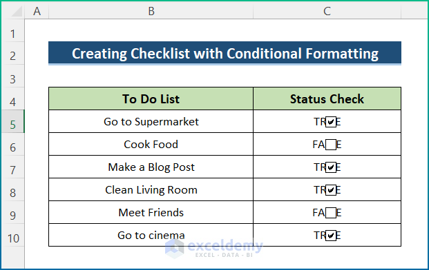
- Furthermore, use a white font color to make them invisible.
Read More: How to Make a Checklist in Excel Without Developer Tab
Step 5: Apply Conditional Formatting on Checklist
- Firstly, select the task range you want to format.
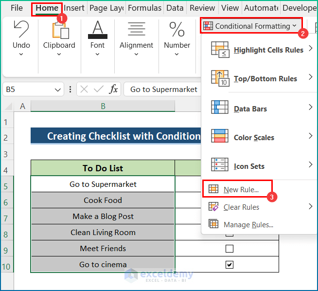
- Secondly, go to the Home tab on your ribbon and select Conditional Formatting from the Styles group section.
- Thirdly, select New Rule from the drop-down menu.
- In the Formatting Rule box, first, select the Use a formula to determine which cells to format option under Select a Rule Type.
- Fourthly, insert the following formula in the Format values where this formula is true.
=C5=TRUE

- After that, click on Format and choose your desired color and format.
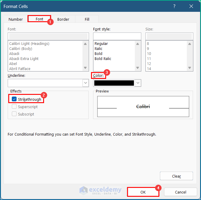
- Lastly, press Ok, and the output will appear as below.
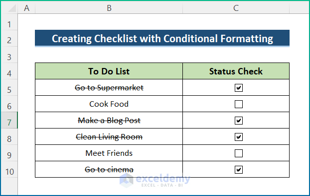
Step 6: Final Checklist with Conditional Formatting
Last but not least, you can make several changes from the Format Cells dialog box. However, the final picture may appear as shown below after some modifications.
💬 Things to Remember
- You can make your checklist more attractive by modifying different options in the Format Cells.
- Afterward, you can choose the checkbox from the list according to your choice.
Download Practice Workbook
You can download the workbook used for the demonstration from the download link below.
Conclusion
These are all the steps you can follow to make a checklist with conditional formatting in Excel. Overall, in terms of working with time, we need this for various purposes. I have shown multiple methods with their respective examples, but there can be many other iterations depending on numerous situations. Hopefully, you can now easily create the needed adjustments. I sincerely hope you learned something and enjoyed this guide. Please let us know in the comments section below if you have any queries or recommendations.
Relative Articles
- How to Create an Audit Checklist in Excel
- How to Create a Drop Down Checklist in Excel
- How to Create an Interactive Checklist in Excel

