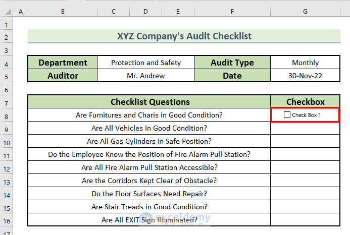
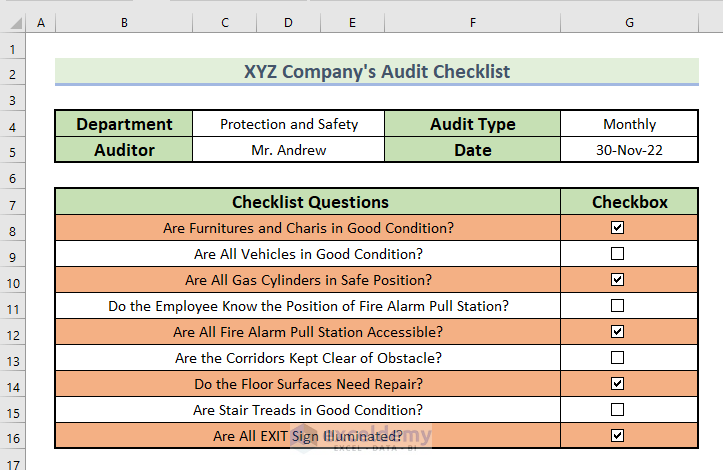
An Overview of an Audit Checklist
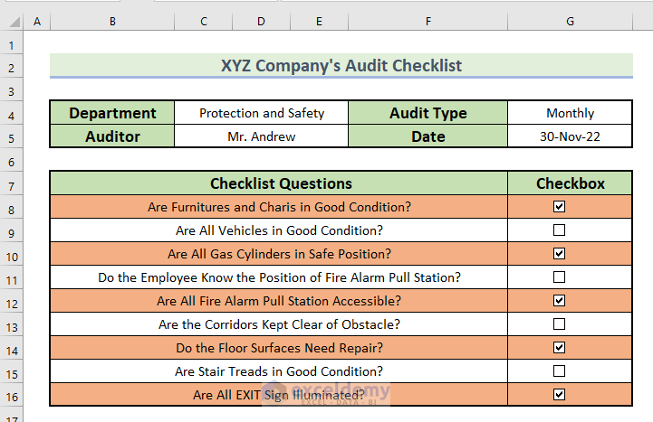
In the following picture, you can see an overview of an Audit Checklist. We will show you how you can create such an audit checklist in Excel.
How to Create an Audit Checklist in Excel: 6 Easy Steps
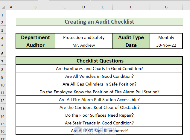
In the following picture, you can see the Checklist Questions for an audit.
Step 1 – Adding the Developer Tab to the Ribbon
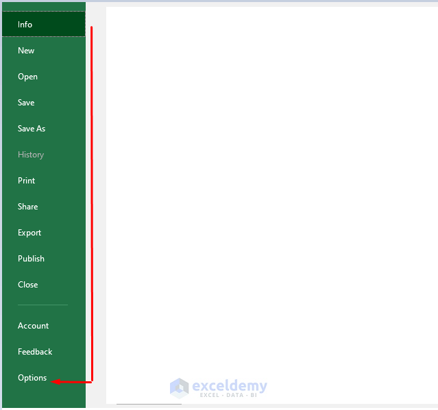
- Go to the File tab.
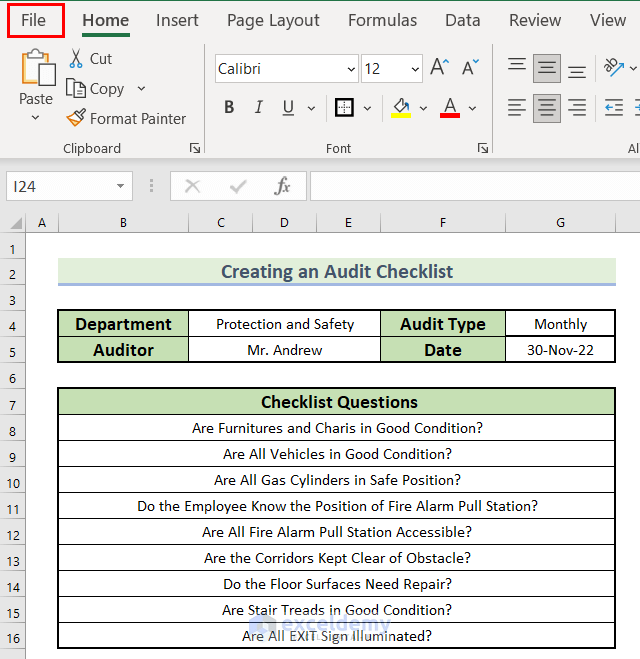
- Select Options.
- From Customize Ribbon, select Developer.
- Click OK.
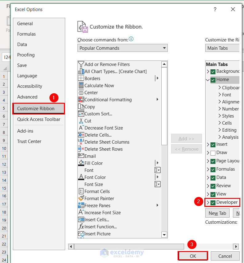
- You will see the Developer tab in the ribbon.
Read More: How to Make a Checklist in Excel Without Developer Tab
Step 2 – Inserting an Interactive Checkbox in Excel
- Go to the Developer tab and select Insert.
- From the Form Controls field, select the Checkbox icon.
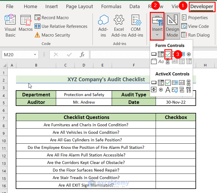
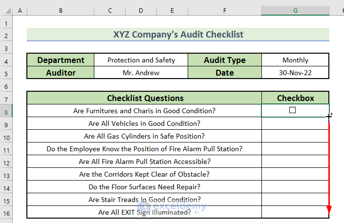
- Put the cursor in the cell where we want to insert the checkbox. We put the cursor in cell G8.
- The cursor will change into a plus (+) sign.
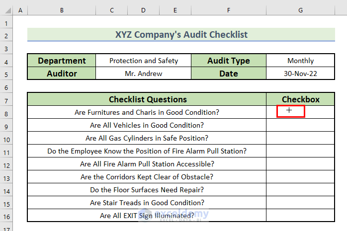
- Click on the cell and the checkbox will appear.
Read More: How to Make a Daily Checklist in Excel
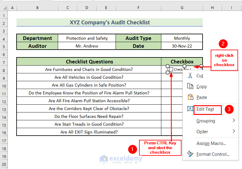
Step 3 – Editing the Checkbox
- Press the Ctrl key and select the checkbox.
- Right-click to open the Context Menu.
- Select Edit Text.
- Select the text with the mouse and press the Backspace key on the keyboard.
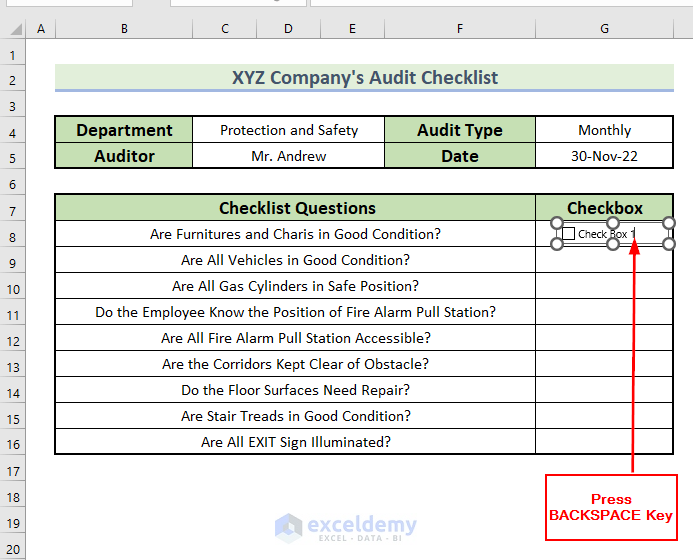
- This will remove the text from the checkbox.
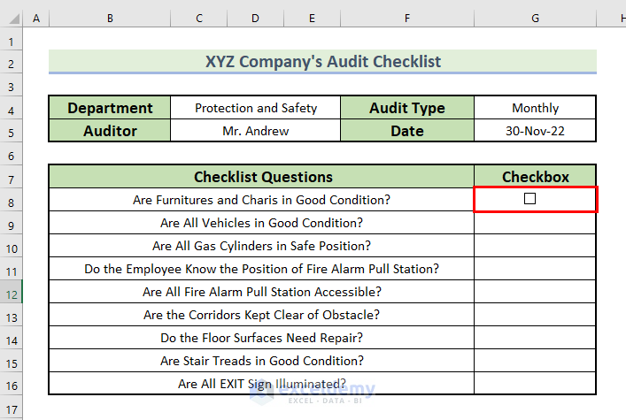
- You can see the checkbox in cell G8.
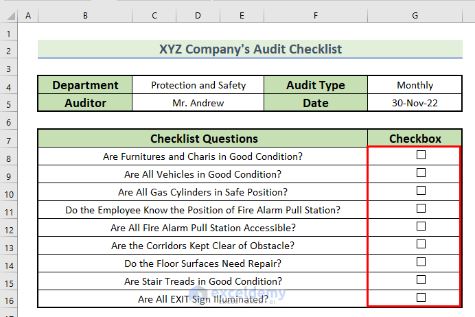
- Copy the checkbox to other cells by dragging down the checkbox with the Fill Handle tool.
- You can see that all the cells from G8 to G16 have a checkbox.
Step 4 – Linking Checkboxes to Cells
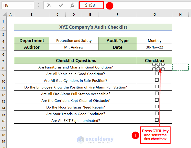
- Press the Ctrl key and select the first checkbox.
- Go to the Formula Bar and insert the following formula.
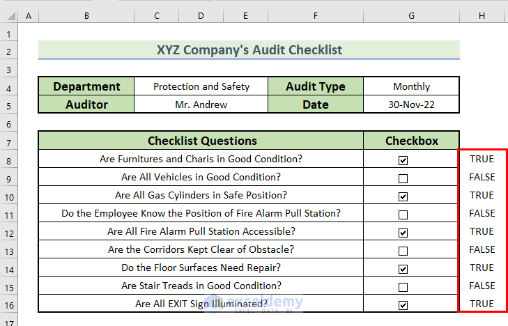
=$H$8- This will link cell H8 with the checkbox of cell G8.
- Since the checkbox of cell G8 is unmarked, cell H8 will show FALSE.
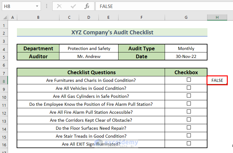
- When we mark the checkbox of cell G8, cell H8 will return TRUE.

Here, we need to type the formula for each individual cell which is time-consuming. Therefore, we will use the VBA code to link the checkbox to a cell, and hence we will find the condition TRUE or FALSE for the Checklist Questions.
Read More: How to Create an Interactive Checklist in Excel
Step 5 -Using VBA to Link Multiple Checkboxes with Checklist
- Press the Alt + F11 keys to open the Visual Basic window. You can also do this from the ribbon: select the Developer tab and choose Visual Basic.

- A VBA Editor window will appear.
- From Insert, select Module.
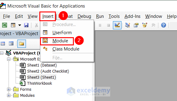
- Copy the following code into the Module.
Sub link_check_boxes_to_cells()
Dim i_check As CheckBox
Dim xcol As Long
xcol = 1
For Each i_check In ActiveSheet.CheckBoxes
   With i_check
     .LinkedCell = _
     .TopLeftCell.Offset(0, xcol).Address
   End With
Next i_check
End Sub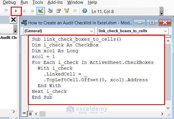
Code Breakdown
- We take link_check_boxes_to_cells as the Sub.
- We declare i_check, and xcol as variables.
- Here, xcol = 1 indicates one column to the right of the checkboxes.
If you want to add one column to the left, type xcol = -1. And if you want to add two columns to the right, type xcol = 2.
- For loop is used to continue the linking of the checkboxes until the last checkbox is found.
- Save the code.
- Run the code. The Run button looks like a play button.
- After closing the Visual Basic window, go back to your worksheet.
- You will see that all checkboxes are linked.
Step 6 – Applying Conditional Formatting in the Audit Checklist
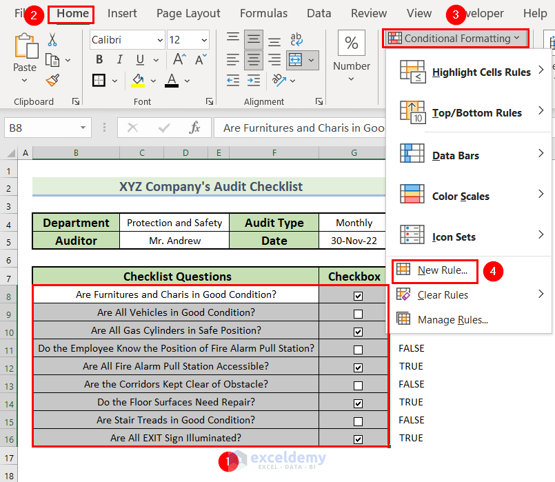
- Select cells B8:G16.
- From the Home tab, select Conditional Formatting.
- Choose New Rule.
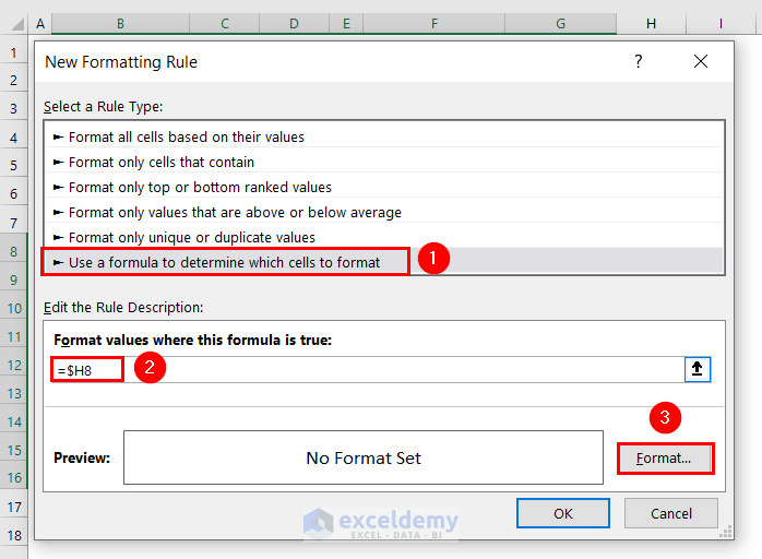
- A New Formatting Rule dialog box will pop up.
- Select Use a formula to detect which cells to format.
- Use the following formula in the Format value where this formula is true box.
=$H8- Click on Format.
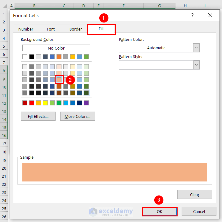
- A Format Cells dialog box will appear.
- From Fill, select a color. We chose a light pink.
- You can see the Sample of the color.
- Click OK.
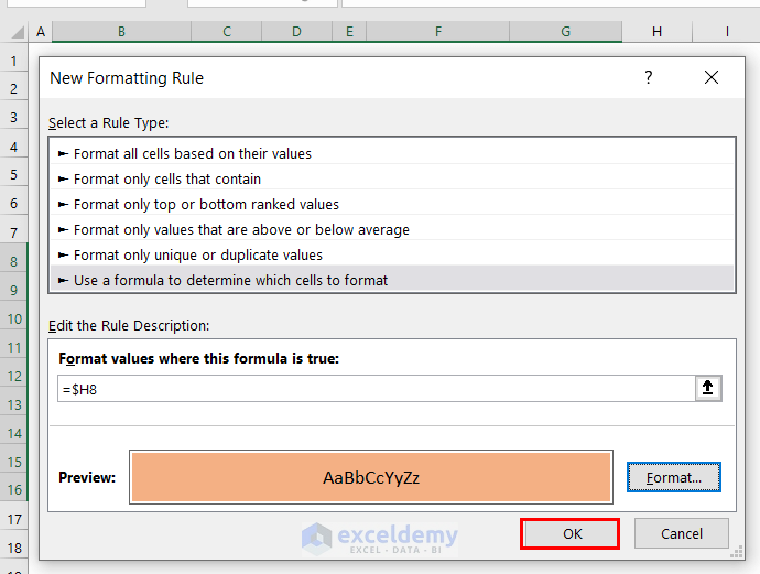
- You can see the Preview of the color. Click OK.
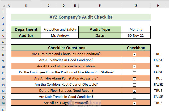
- The marked checklists along with their Checklist Questions are highlighted with light pink color.
We do not need to show the TRUE and FALSE values in the Audit Checklist.
- Select cell H8:H16 and go to the Home tab.
- From the Font group, select Font Color.
- Select While as the Font Color to make the cells invisible.
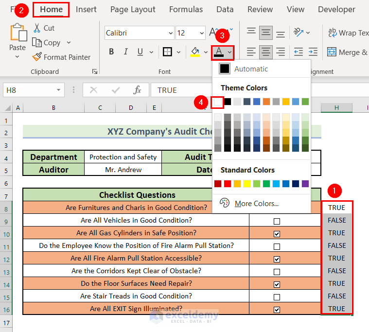
- The audit checklist looks more eye-catching.
Read More: How to Make Checklist with Conditional Formatting in Excel
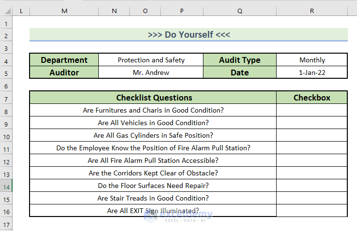
Practice Section
You can download the Excel file to practice the explained method.
Download the Practice Workbook


Alssalaam
I was looking for how auditors can schedule their audit workload, assign resources like human resources,time etc to meet audit deadlines.
In the process your website came up. However the topic is different.
Can you address the topic i was looking for?
Many thanks
Hello AM!
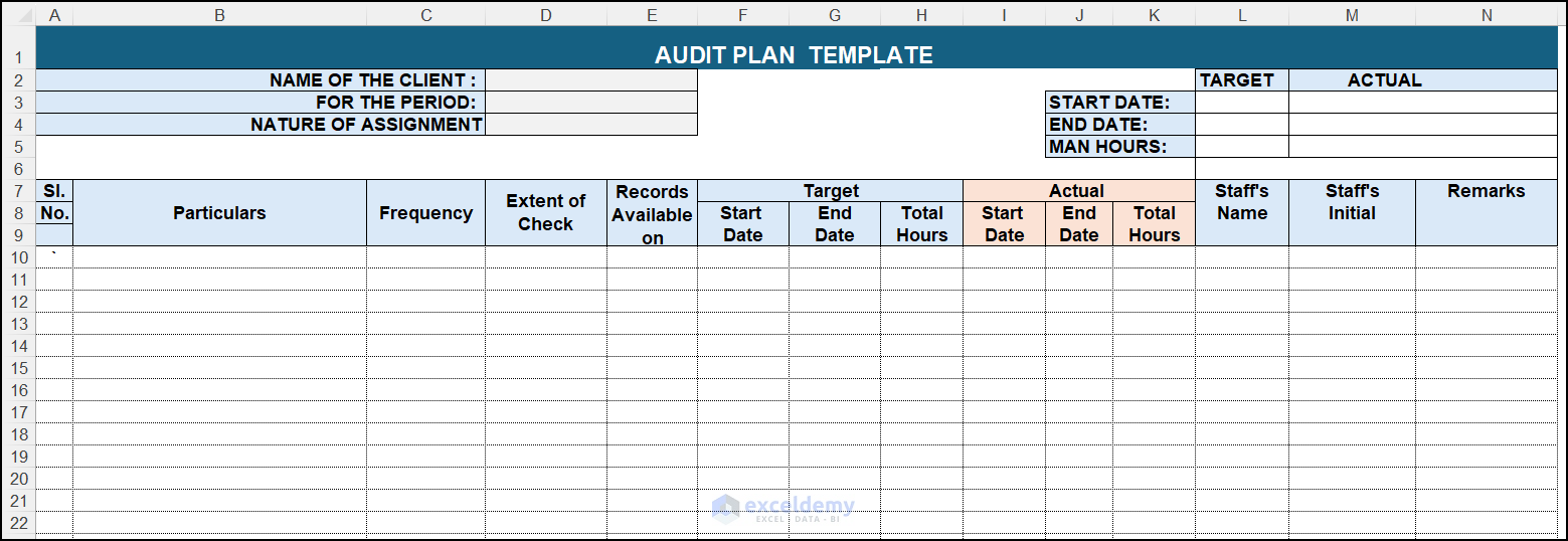
Thanks for your comment. To schedule the audit workload and assign resources, you can create an Audit Plan Template. To do this, you have to assign these parameters. I am listing the items with proper descriptions:
1. Particulars: This column should describe the specific audit item or task that needs to be checked or reviewed. It could be a process, financial statement, or any other aspect of the audit.
2. Frequency: This column specifies how often the particular item is audited. For example, it might be done annually, quarterly, monthly, or as needed.
3. Extent of Check: This column outlines the depth or scope of the audit procedure. It could be a high-level review or any other specified level of scrutiny.
4. Records Available On: This column indicates where the relevant records or documents are available. 5. Target Start and End Date: These columns define the planned dates for starting and completing the audit procedure for the particular item.
6. Actual Start and End Date: These columns record the actual dates when the audit procedure for the specific item started and ended.
7. Total Hours: This column can be used to record the total number of hours spent on auditing the particular item.
8. Staff’s Name: This column mentions the name of the staff or auditor responsible for conducting the audit for the particular item.
9. Staff’s Initial: This column can be used for the staff member’s initials or code for identification purposes.
10. Remarks: This column allows auditors to provide comments or notes related to the audit of the specific item. This can include observations, findings, issues, or any other relevant information.
Here, you can see the image of the template that I have made for you. Also, you can download the template from the following link.