How to Create a Drop Down Checklist in Excel (with Quick Steps)

Excel is a fantastic tool for working with extensive data and user inputs. When working with user inputs, it is a frequent scenario in which the users are needed to choose options or list things. In this regard, creating a drop-down checklist is a magnificent approach. In this article, I will show you all the steps to create a drop-down checklist in Excel.

How to Create a Drop Down Checklist in Excel: Step-by-Step Procedures

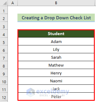
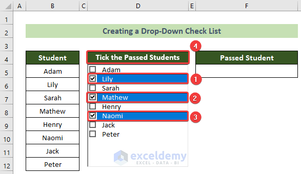
Say, we have a dataset of several students’ names. Now, of these students, only 3 passed. Now, we want to create a drop-down checklist containing these students’ names. Then, we want to check the passed students’ names and get an output in another cell containing only the passed students.

Follow the step-by-step guidelines below to accomplish this result.

📌 Step 1: Create Drop Down Checklist Options

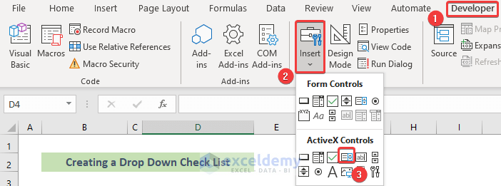
To create a drop-down checklist, the first thing that you need to do is to create the drop-down checklist options.

To do this, first and foremost, click on the Developer tab on your Excel ribbon.
Following, click on the Insert tool >> ActiveX Controls group >> List Box (ActiveX Control) option.

As a result, a list box will be in your control.
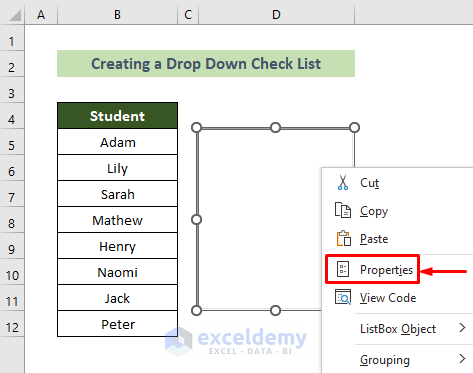
Now, drag your mouse to determine the list box area.
Following, right-click on the list box area and choose the Properties option from the context menu.

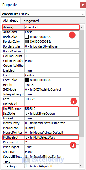
Consequently, a Properties window will appear.
Following, write checkList in the (Name) text box.
Subsequently, refer to the cells B5:B12 in the ListFillRange text box.
Following, choose option 1 – fmListStyleOption from the ListStyle option list.
Last but not least, choose option 1 – fmMultiSelectMulti from the MultiSelect option list.

Thus, there will be a drop-down checkbox list with the student’s names.
Now, to get the passed students’ names in a cell, create a header and name the output cell as CheckListOuput in the NameBox.

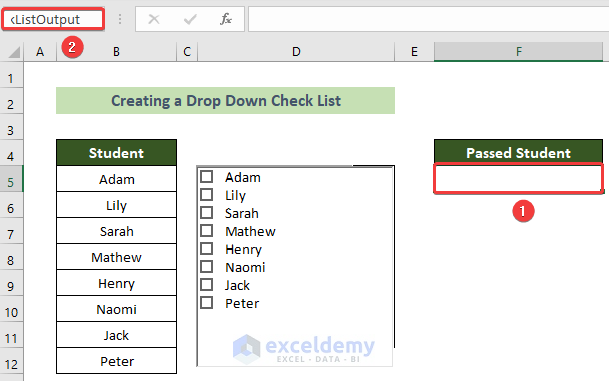
As a result, your dropdown checklist options are created properly and the output cell is also declared with a proper name.

📌 Step 2: Add an Interactive Button to Extract the Result

Now, you need to add a button to make a checklist interactive and extract your desired result.

In order to do this, first, go to the Insert tab.
Following, go to the Illustrations group >> Shapes tool >> Rectangle option.

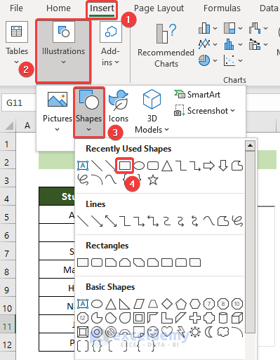
As a result, you will have control over a rectangle now.
So, drag your mouse to create your button area and fill the rectangle with your desired color.
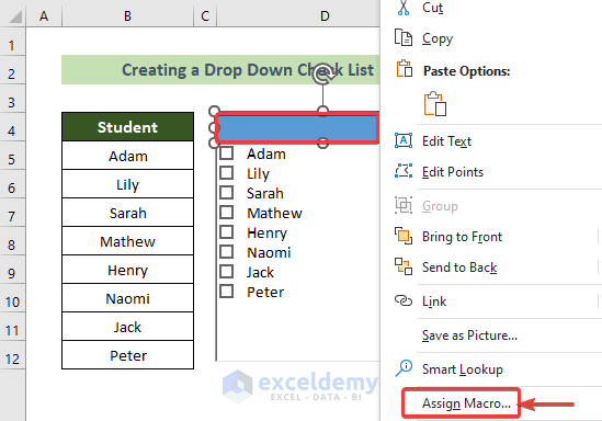
Afterward, right-click on your mouse inside the rectangle area and choose the Assign Macro… option from the context menu.

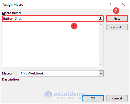
As a result, the Assign Macro window will appear.
Now, name your macro as Button_Click on the Macro Name: option and click on the New button.

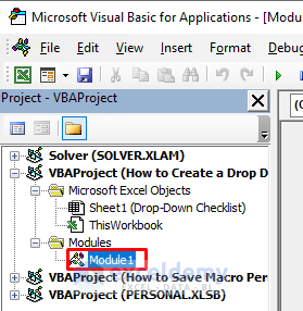
Consequently, the VB Editor will open automatically creating a new module named Module1.

Now, inside the module’s code window, write the following VBA code.

Sub Button_Click()
Dim buttonShape As Shape, listOption As Variant, M, N As Integer
Dim xP As String
Set buttonShape = ActiveSheet.Shapes(Application.Caller)
Set checkListBox = ActiveSheet.checkList
If checkListBox.Visible = False Then
    checkListBox.Visible = True
    buttonShape.TextFrame2.TextRange.Characters.Text = "Tick the Passed Students"
    resultStr = ""
    resultStr = Range("CheckListOutput").Value
    
    If resultStr <> "" Then
         resultArr = Split(resultStr, ";")
    For M = checkListBox.ListCount - 1 To 0 Step -1
        xP = checkListBox.List(M)
        For N = 0 To UBound(resultArr)
            If resultArr(N) = xP Then
              checkListBox.Selected(M) = True
              Exit For
            End If
        Next
    Next M
    End If
Else
    checkListBox.Visible = False
    buttonShape.TextFrame2.TextRange.Characters.Text = "Click Here"
    For M = checkListBox.ListCount - 1 To 0 Step -1
        If checkListBox.Selected(M) = True Then
        listOption = checkListBox.List(M) & ";" & listOption
        End If
    Next M
    If listOption <> "" Then
        Range("CheckListOutput") = Mid(listOption, 1, Len(listOption) - 1)
    Else
        Range("CheckListOutput") = ""
    End If
End If
End Sub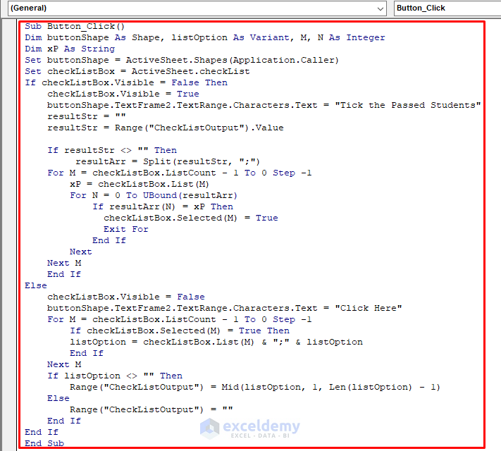

Note:

In the code, the button’s macro name is Button_Click; checkList is the name of our checklist, and checkListOutput is the output cell’s name.

You must change these names inside the VBA code if you name these things something else.

Afterward, press Ctrl + S on your keyboard.
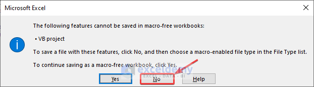
As a result, a Microsoft Excel window will appear.
Following, click on the No button.

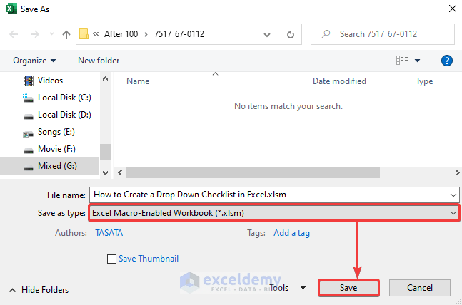
Consequently, the Save As dialogue box will appear.
Following, choose the Save as type: option as .xlsm file and click on the Save button.

Thus, the code is saved and workable now.
At this time, close the code window and go back to your main Excel file.
You will see there will be interactive checkboxes and the Tick the Passed Students button.
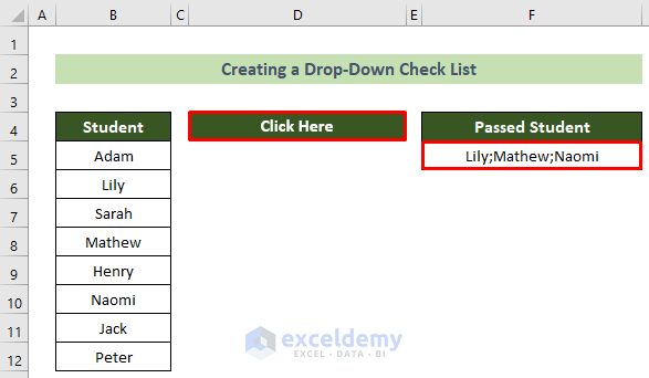
Now, click on the passed students’ names Lily, Mathew, and Naomi.
Following, click on the Tick the Passed Students button.

As a result, you will find your result in cell F5 and the button will be named Click Here now interactively.

Thus, you will be able to create a drop-down checklist in Excel and will be able to use the checklist to generate results.

Download Practice Workbook

You can download our practice workbook from here for free!

How to Create a Drop Down Checklist.xlsm

Conclusion

So, in this article, I have shown you step-by-step guidelines to create a dropdown checklist in Excel. You can also download our free workbook to practice. I hope you find this article helpful and informative. If you have any further queries or recommendations, please feel free to comment here.

Have a nice day! Thank you!

Relative Articles

Get FREE Advanced Excel Exercises with Solutions!