Dataset Overview
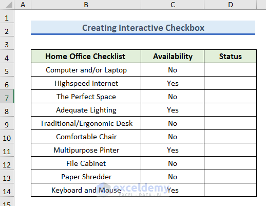
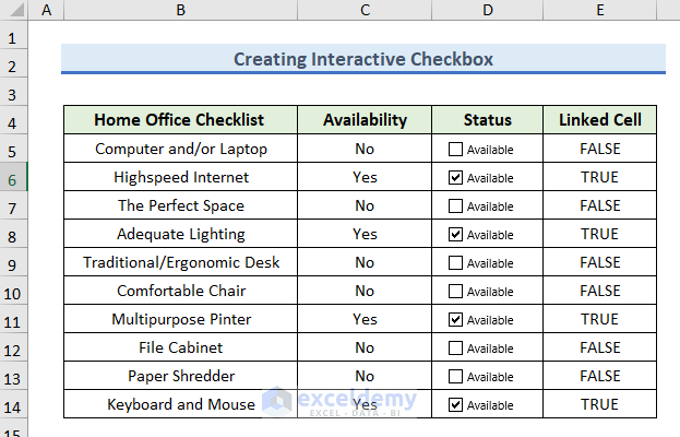
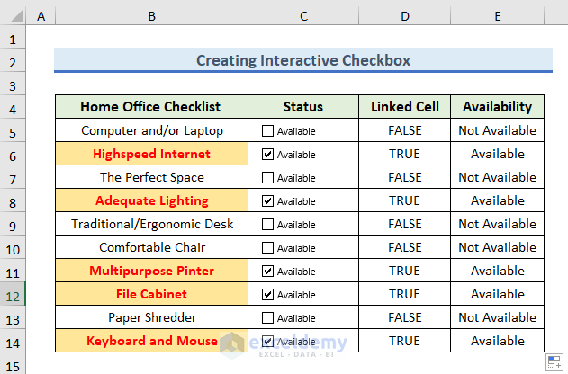
To demonstrate the steps, we will use the dataset of the Home Office Checklist with answers. In Column B, we have information about a list of products necessary for the home office. In Column C, we have information about the product’s availability. Let’s follow the steps to learn how we can create an interactive checklist in Excel.

Step 1 – Enable the Developer Tab
- If the Developer tab isn’t visible in the ribbon, follow these steps:
- Click the File tab.
-
- In the bottom-left corner, select Options.
-
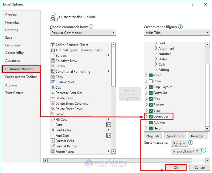
- In the Excel Options window, choose the Customize Ribbon section.
- Check the Developer option and press OK.
Read More: How to Make a Checklist in Excel
Step 2 – Insert a Checkbox
- Create a new column called Status.
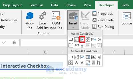
- Go to the Developer tab and select Insert.
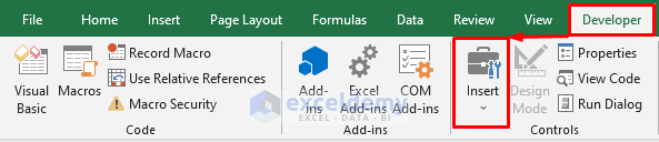
- Click the Checkbox icon in the Form Controls section.
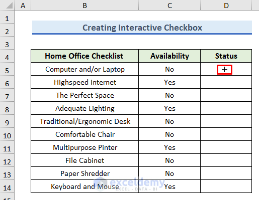
- You will see a (+) sign.
- Click cell D5 to insert the checkbox.
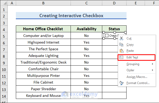
- Right-click the checkbox, select Edit Text, and name it (e.g., Available).
Read More: How to Make a Checklist in Excel Without Developer Tab
Step 3 – Add Multiple Checkboxes in Excel
- Use the Fill Handle to drag down from cell D5 to create checkboxes for each item.

Read More: How to Make a Daily Checklist in Excel
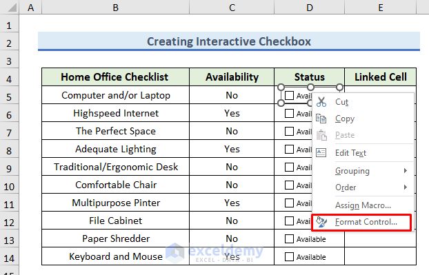
Step 4 – Link Cells with Checkboxes
- Right-click the checkbox in cell D5 and choose Format Control.
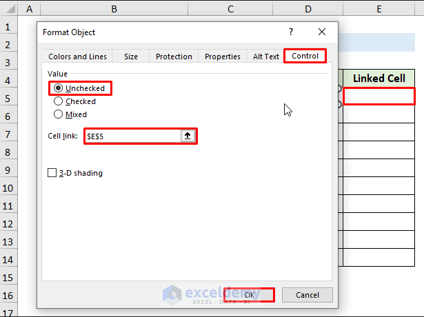
- In the Format Object window, go to the Control tab.
- Check Unchecked and set the Cell Link to $E$5.
- Click OK.
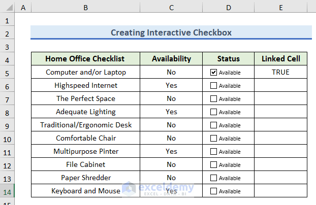
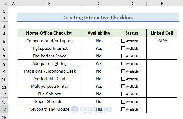
- When the checkbox in D5 is ticked, cell E5 will show TRUE, and unticked will show FALSE.
- Repeat this process for other cells (E6 to E14) to link checkboxes in columns D and E.
Read More: How to Create a Drop Down Checklist in Excel
Step 5 – Make Interaction with Checklist
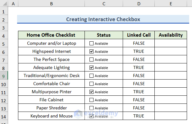
- Delete the elements in the Availability column and move it to column E.
- We’ll demonstrate how the Availability column can be controlled by the checkboxes.
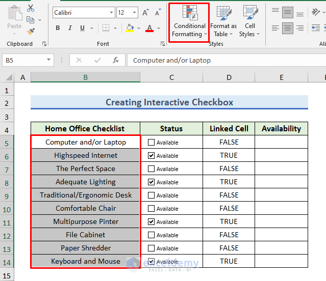
- Select cells from B5 to B14.
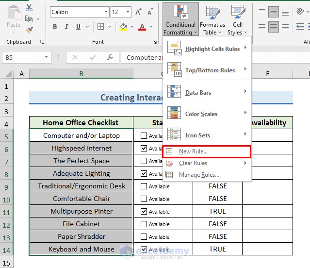
- Go to the Conditional Formatting option in the ribbon.
- Choose New Rule.
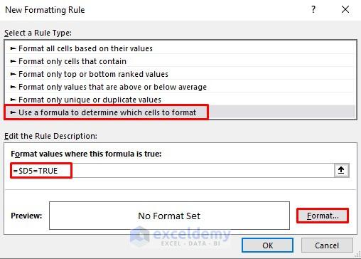
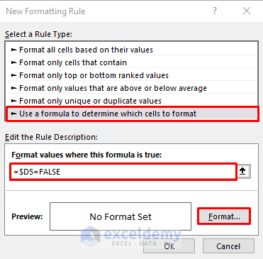
- In the New Formatting Rule window, select Use a formula to determine which cells to format.
- Enter the formula:
=$D5=TRUE- Click Format to change the format in the Home Office Checklist column.
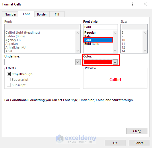
- In the Format Cells window, choose a bold font style and set the font color to red.
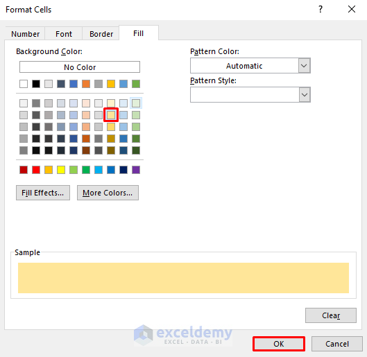
- Go to the Fill tab and select a background color.
- Confirm the changes by clicking OK.
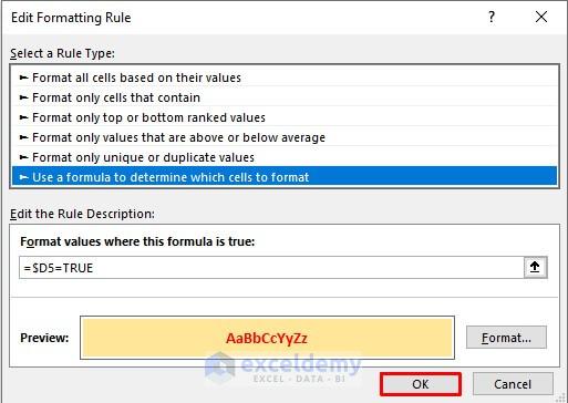
- In the New Formatting Rule window, you can see the preview.
- Press OK.
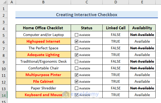
- Now, when the checkbox is ticked, column B will show the modified format.
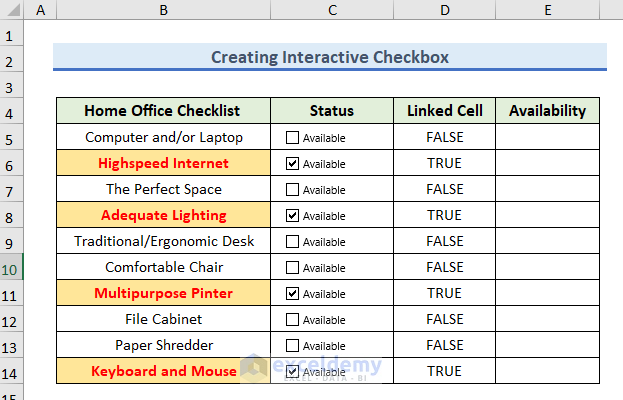
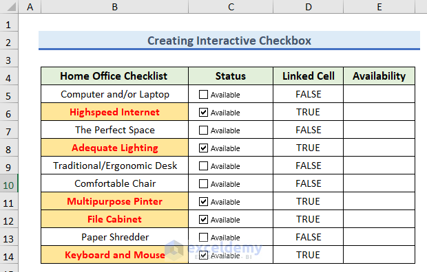
- Suppose we have bought a File Cabinet.
- We will put a tick on File Cabinet.
- Linked Cell and Home Office Checklist columns have changed as the checklist is interlinked.
Read More: How to Make Checklist with Conditional Formatting in Excel
Step 6 – Link Checklist with Availability
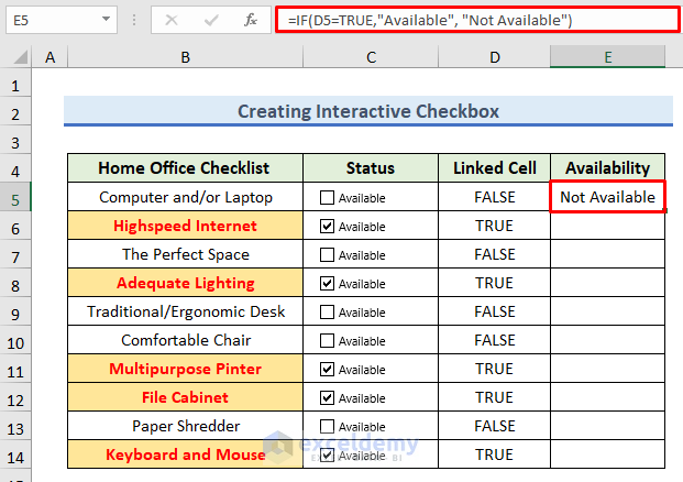
- In column E, we want to show Available or Not Available based on the checkbox status.
- In cell E5 enter the formula:
=IF(D5=TRUE,"Available","Not Available")- The result in cell E5 shows Not Available.
- Apply the same formula to all cells in the Availability column using the Fill Handle.
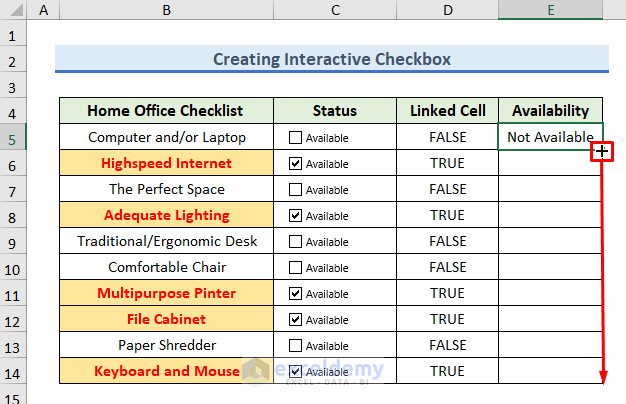
- The output is visible.
Read More: How to Create an Audit Checklist in Excel
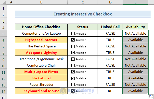
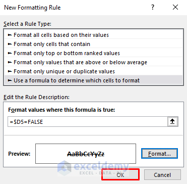
Step 7 – Format Fonts of Availability Column
- Select cells from E5 to E14.
- Go to Conditional Formatting and choose New Formatting Rule.
- Enter the formula:
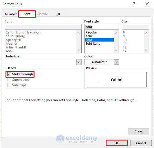
=$D5=FALSE- Click Format and select formatting options (e.g., bold font style and strikethrough effect).
- Confirm the changes by clicking OK.
- The preview is showing in the preview box.
- Press OK.
- The modification is visible, with Not Available showing with strikethrough.
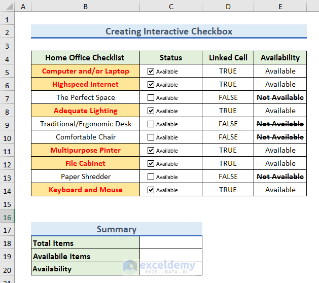
Step 8 – Insert Summary Based on Checklist
- Tick Computer and/or Laptop and observe the changes.
- Add a summary:
-
- Total Items:
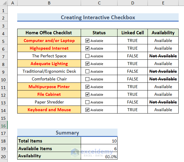
- Enter the following formula in cell C18:
- Total Items:
=COUNTA(B5:B14)-
- Available Items:
- Insert the following formula in cell C19:
- Available Items:
=COUNTIF(D5:D14,TRUE)-
- Availability Percentage:
- Enter the following formula:
- Availability Percentage:
=C19/C20- Change the format to Percentage by pressing Ctrl + 1.
- The summary now displays information about total items, available items, and availability percentage.
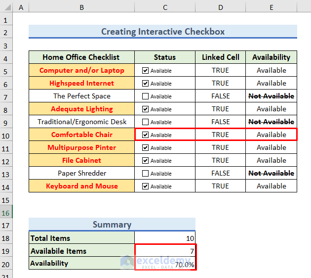
Final Output
- Ticking Comfortable Chair will change the format of the Home Office Checklist column.
- The Availability column reflects item availability.
- The summary shows increased available items and availability percentage.
- Our checklist is interactive, interacting with other data.
You can download the practice workbook from here:
Get FREE Advanced Excel Exercises with Solutions!

