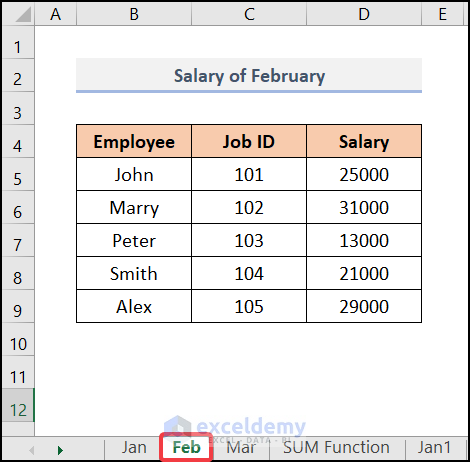
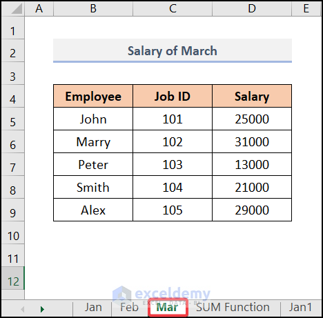
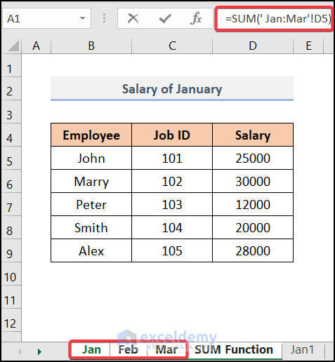
Here we use three worksheets on the Salary of Employees for January, February, and March. We used the short form of the month names as the sheet name. Let’s use formulas that take data from these sheets simultaneously.

Method 1 – Calculating a Sum Across Multiple Sheets
Case 1.1 – Left-Clicking on the Sheet Tab
Steps:
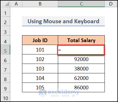
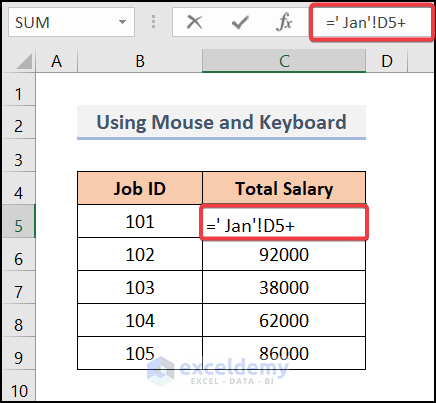
- In a separate sheet, choose cell C5 to store the sum of the first employee’s salary.
- In cell C5, insert an equals (=) sign. Don’t press Enter yet.
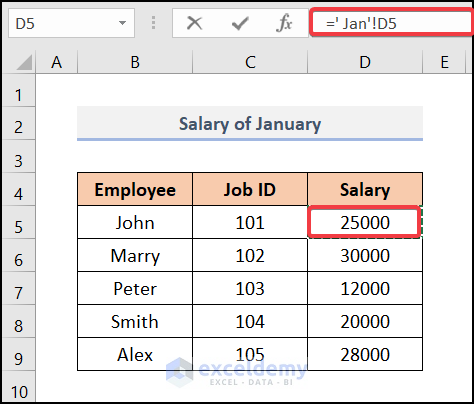
- Go to the first sheet named Jan and select cell D5 of the salary.
- Insert a plus sign (+).
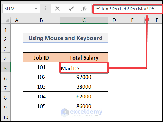
- Add the data from other sheets using the same procedure.
- After adding all the sheets your formula bar will look like the image below.
- Press Enter.
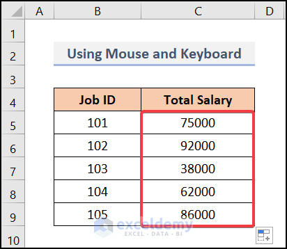
- Drag down the Fill Handle.
Case 1.2 – Using the SUM Function
Steps:
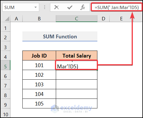
- Create a new worksheet where you want to calculate the sum results.
- Go to the worksheet named Jan and select the cell you want to add.
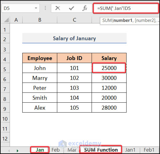
- Go to the last sheet of your file. We chose the Mar sheet, and now we will add the Sheets.
- Apply the following formula in cell C5 in the new sheet:
Here, the syntax SUM(‘ Jan: Mar’!D5) will add all the D5 cells of your corresponding worksheets.
- Press Enter.
- Drag down the Fill Handle tool for the other cells.
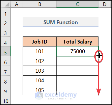
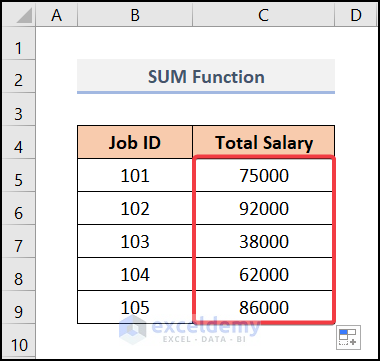
- You will get the final results.
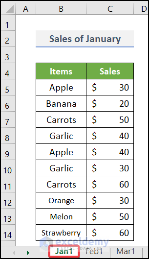
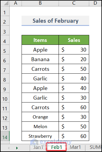
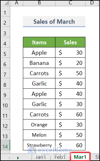
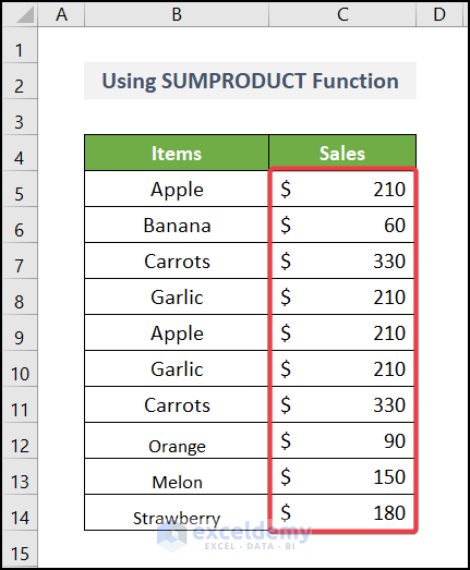
Case 1.3 – Utilizing the SUMPRODUCT Function
For this method, we’ll use three datasets of Items Sales for three months.
Steps:
- Go to the a worksheet where you want to calculate the total sum.
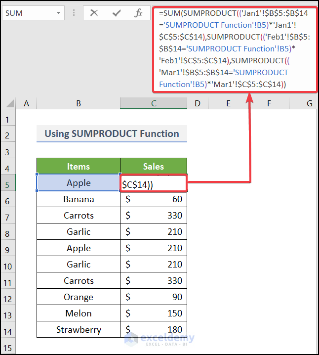
- Copy the formula below.
Formula Breakdown:
SUMPRODUCT((‘Jan1′!$B$5:$B$14=’SUMPRODUCT Function’!B5)*’Jan1′!$C$5:$C$14)→ The SUMPRODUCT function takes the whole range of Jan1 as Jan1′!$B$5:$B$14 and returns TRUE for the corresponding cell value of B5. Otherwise, it will return FALSE for cell B5 where the text is Apple. Now it starts to find the actual match from Jan1′!$C$5:$C$14 range and returns the value 70 for cell B5.
The same formula was applied to the other sheets also.
SUM(SUMPRODUCT((‘Jan1′!$B$5:$B$14=’SUMPRODUCT Function’!B5)*’Jan1′!$C$5:$C$14),SUMPRODUCT((‘Feb1′!$B$5:$B$14=’SUMPRODUCT Function’!B5)*’Feb1′!$C$5:$C$14),SUMPRODUCT((‘Mar1′!$B$5:$B$14=’SUMPRODUCT Function’!B5)*’Mar1′!$C$5:$C$14))→ The SUM function will add the return value of the SUMPRODUCT function eventually.
- Apply the formula to the first cell in the result column.
- Press Enter.
- Use AutoFill for the other cells in the column.
Read More: How to Apply Same Formula to Multiple Cells in Excel
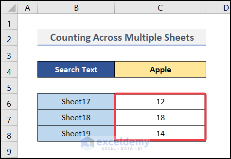
Method 2 – Counting Across Multiple Sheets
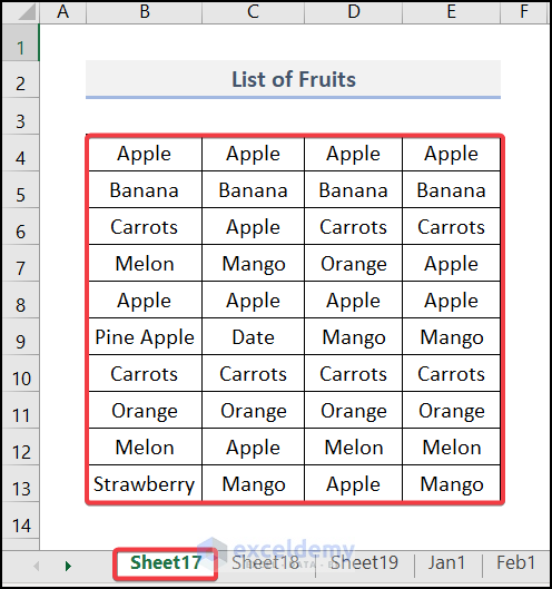
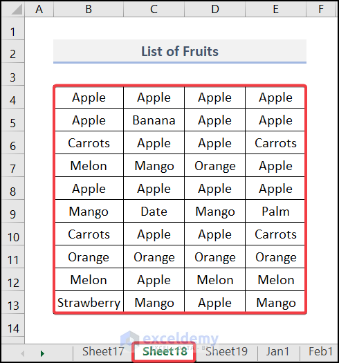
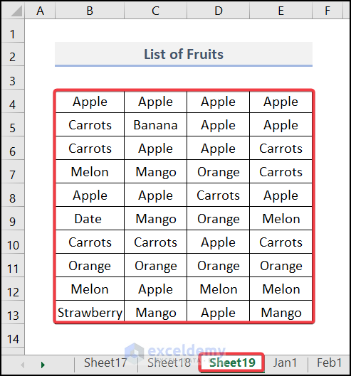
Let’s assume you have several datasets where the same values repeat across the tables. You want to count how many times a specific item appears in the sheets. We’ll use a List of Fruits and count how many times the word Apple appears in our datasets.
Steps:
- Pick cell C6 in a new sheet and copy the following formula inside.
=COUNTIF(INDIRECT(“‘”&B6&”‘!”&”B4:E13”),$C$4)
Here,
C4= The searched value that you want to count.
B6= The corresponding sheet name.
B4:E13= The range of the dataset you want to count.
Formula Breakdown:
INDIRECT(“‘”&B6&”‘!”&”B4:E13”)→ It took the value of the cell B4:E13 as a reference value and returns the value in cell B6. Here B6 cell refers to sheet17.
COUNTIF(INDIRECT(“‘”&B6&”‘!”&”B4:E13”),$C$4)→ $C$4 is the cell where you inserted the value that you want to count. It took the text string Apple and count for the referred range value of the INDIRECT function. The final output here is 12 which is the total count for the inserted text Apple in sheet17.
- Press Enter.

Note: The COUNTIF function is not a case-sensitive function.
- AutoFill to the other cells in the column.
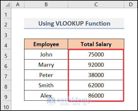
Method 3 – Applying Formula to Lookup Values
Case 3.1 – Using the VLOOKUP Function
Steps:
- Select the cell C5 and enter the following formula:
Here,
B5= The cell for whom you want to find out the corresponding value
B5:D9= The entire range of each worksheet.
Formula Breakdown:
VLOOKUP(B5,’ Jan’!$B$4:$D$9,{3}, FALSE)→ the VLOOKUP function finds the value identical to cell B5 of the Employee column. It searches into the table array of Jan worksheets ($B$4:$D$9) and then takes the col_index_num {3} which is the Salary column. False returns the exact value from the column.
VLOOKUP(B5,’Jan’!$B$4:$D$9,{3},FALSE),VLOOKUP(B5,Feb!B5:D9,{3},FALSE),VLOOKUP(B5,Mar!B5:D9,{3},FALSE)→ This function will repeat the same formula stated above for the other sheets.
SUM(VLOOKUP(B5,’Jan’!$B$4:$D$9,{3},FALSE),VLOOKUP(B5,Feb!B5:D9,{3},FALSE),VLOOKUP(B5,Mar!B5:D9,{3},FALSE))→ The sum function will add all the value that the VLOOKUP function returns after finding out.
- Output→ 25000+25000+25000=75000.

- Press Enter and drag down Autofill for other cells to get the rest of the results.
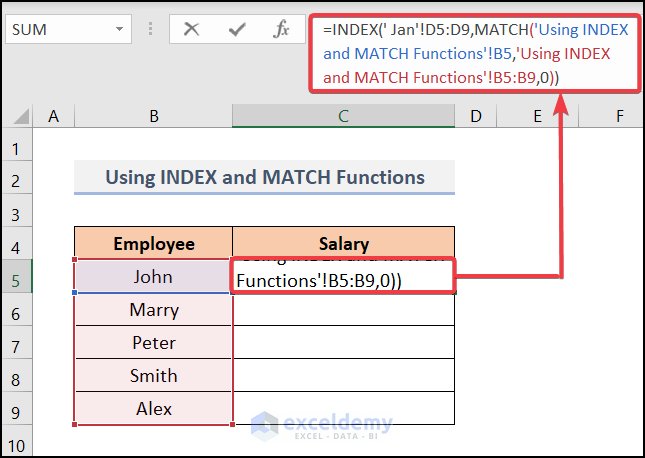
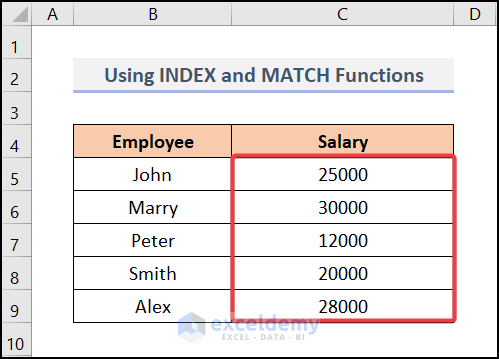
Case 3.2 – Using INDEX and MATCH Functions
Steps:
- Select cell C5 of your main worksheet where you want to find out the looking value and apply the following formula in it:
Formula Breakdown:
MATCH(‘Using INDEX and MATCH Functions’!B5,’ Using INDEX and MATCH Functions’!B5:B9,0)→ The MATCH function finds the location of the value from cell B5 in the current worksheet from cells B5:B9.
- Output→9,1
INDEX(‘ Jan’!D5:D9, MATCH(‘Using INDEX and MATCH Functions’!B5,’ Using INDEX and MATCH Functions’!B5:B9,0))→ Then the INDEX function evaluates the matched value for the worksheet Jan’!D5:D9 and returns their corresponding value.
- Output→25000
- Drag down the Fill Handle tool with the same formula for the other cells.
Read More: How to Use Multiple Excel Formulas in One Cell
Practice Section
We have provided a practice section on each sheet on the right side so you can use these methods and experiment.
Download Practice Workbook
Download the following practice workbook.
Related Articles
- How to Apply Formula to Entire Column Without Dragging in Excel
- How to Exclude Zero Values with Formula in Excel
- How to Make FOR Loop in Excel Using Formula
- How to Apply Formula to Entire Column Using Excel VBA
<< Go Back to How to Create Excel Formulas | Excel Formulas | Learn Excel
Get FREE Advanced Excel Exercises with Solutions!
