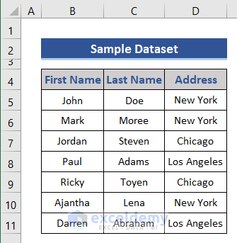
This is the sample dataset.
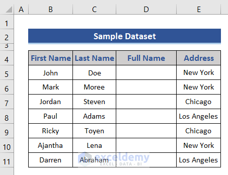
To concatenate the First Name and Last Name:
Method 1. Combine Names in Two Columns with Space/Comma/Hyphen Using an Excel Formula
i. Using the Ampersand Operator
Steps:
- Enter the formula using the ampersand in D5.
=B5&" "&C5
- B4 and C4 are the cell references of the first row from First Name and Last Name columns.
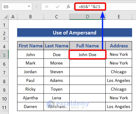
Between the ampersands there is a " ". to use a space to separate the two names.
The first name (cell reference) was entered, the space was added using an ampersand and the second ampersand concatenated the last name.
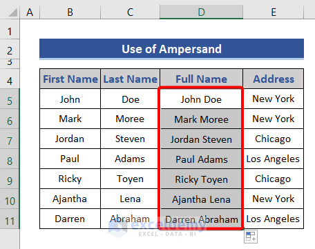
- Drag down the Fill Handle to see the result in the rest of the cells.
To combine two columns with a comma or hyphen instead of a space, use the following formulas.
For Comma:
=B5&","&C5
For Hyphen:
=B5&"-"&C5
ii. Using the Excel CONCATENATE Function
Steps:
- Enter the formula.
=CONCATENATE(B5," ",C5)
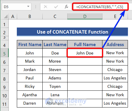
Space: " " is the second text (text2) in the function.
- Drag down the Fill Handle to see the result in the rest of the cells.

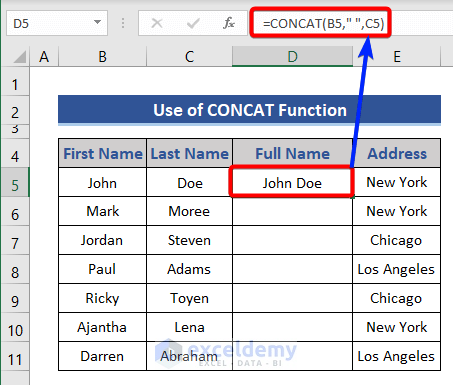
iii. Use the CONCAT Function to Concatenate Columns
Steps:
- Enter the formula.
=CONCAT(B5," ",C5)
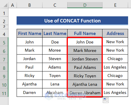
- Drag down the Fill Handle to see the result in the rest of the cells.
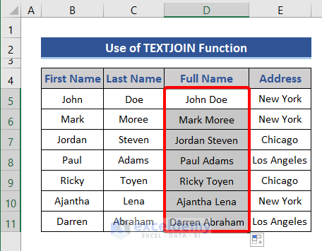
iv. Using the TEXTJOIN Function to Concatenate Two Columns
Steps:
- Enter the formula.
=TEXTJOIN(" ",1,B5,C5)
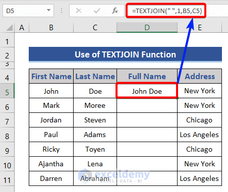
The space (" ") is set as delimiter. Empty cells are ignored, using 1 in the second parameter.
- Drag down the Fill Handle to see the result in the rest of the cells.
Read More: How to Merge Two Columns in Excel
Method 2 – Concatenate Two Columns Using the Flash Fill Feature
Steps:
- Enter a name manually.
- Select the cell.
- In the Data tab, select Data Tools.
- Click Flash Fill.
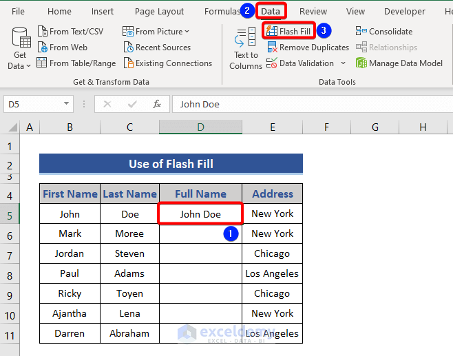
This is the output.
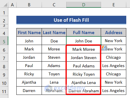
You can also press Ctrl+E to use the Flash Fill.
How to Concatenate Values of Two or More Columns in Excel with a Line Break
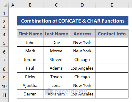
To find the Contact Info:
Steps:
- Use CONCAT function with the CHAR function.
=CONCAT(B5," ",C5,CHAR(10),D5)
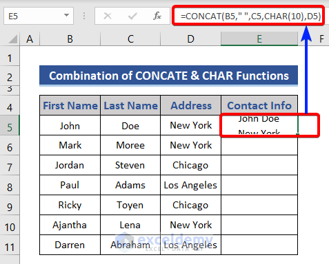
CHAR(10) is used for a line break. The address is joined with a line break.
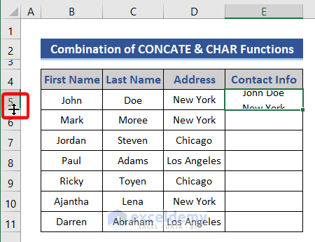
- Adjust the height of Row 5.
- Go to the row number bar. Place the cursor between Rows 5 and 6.
- Double-click.
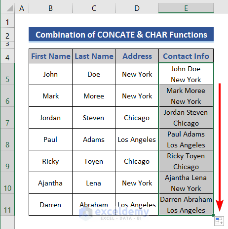
- Drag down the Fill Handle to see the result in the rest of the cells.
Download Practice Workbook
Download the practice workbook.
Merge Columns in Excel: Knowledge Hub
<< Go Back to Merge in Excel | Learn Excel
Get FREE Advanced Excel Exercises with Solutions!
