In this article, I’m going to explain how to Calculate Simple Interest Loan Payments in Excel. Here, I have described five methods of calculating Simple Interest Loan Payments in Excel.
What Is a Simple Interest Loan Payment?
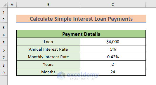
Simple interest is a constant interest rate that is calculated on a loan. In the case of simple interest loan payments, you have to pay a fixed interest rate on the loan monthly.
To explain the 5 methods on how to calculate simple interest loan payments in Excel, I have used the following dataset. Which contains two columns with Payment Details.
1. Applying PMT Function to Calculate Simple Interest Loan Payments in Excel
We can apply the PMT function to calculate simple interest loan payments in Excel. PMT function is a built-in function in Excel.
Steps:
- Firstly, select a different cell C11 where you want to calculate the Monthly Payment.
- Secondly, use the corresponding formula in the C11 cell.
=PMT(C7,C9,-C5)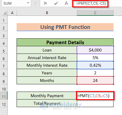
Formula Breakdown
Here, I have used the PMT function which calculates the payment based on a loan with a constant interest rate and regular payment.
- In this function, C7 denotes the monthly interest rate of 0.42%.
- C9 denotes the total payment period in terms of the month which is 24.
- C5 denotes the present value which is $4000.
- At this time, press ENTER to see the amount of the Monthly Payment.

Next, I will calculate the Total Payment.
- Now, type the following formula in cell C12.
=C11*C9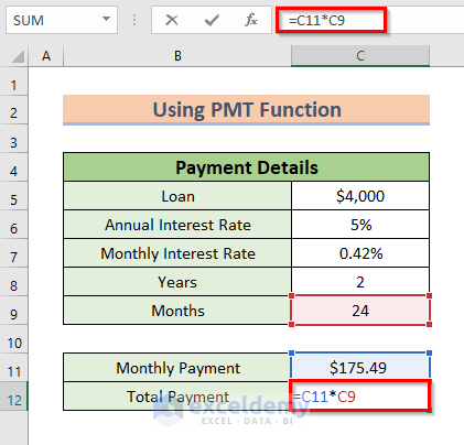
Here, in this formula, I multiplied the Monthly Payment by the total Months.
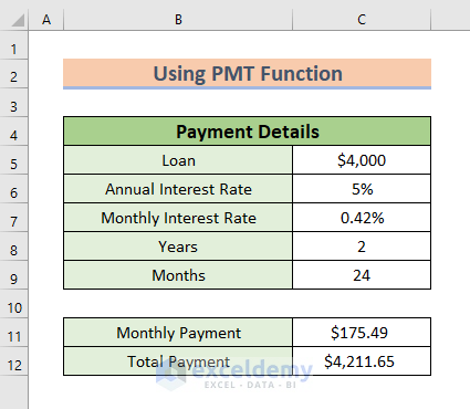
- Now, press ENTER to see the amount of the Total Payment.
As a result, you will get the Total Payment of the Loan amount.
Read More: Convert Compound Interest to Simple Interest in Excel
2. Using PMT & POWER Functions for Determining Simple Interest Loan Payments
I can use PMT and POWER functions to calculate the simple interest loan payments. The steps are given below-
Steps:
- First, select a different cell C11 where you want to calculate the Monthly Payment.
- Then, use the corresponding formula in the C11 cell.
=PMT(POWER((1+C6/C7),(C7/12))-1,C9,C5)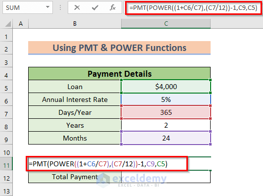
Formula Breakdown
- POWER((1+C6/C7),(C7/12))—-> The POWER function contains a variable and raises it to fixed power.
- POWER((1+0.000136986301369863),30.4166666666667)—-> becomes
- POWER(1.00013698630137,30.4166666666667)—-> turns into
- Output: 1.0041750727376
- PMT(POWER((1+C6/C7),(C7/12))-1,C9,C5)—-> The PMT function gives the payments on the loan with a constant interest rate.
- PMT(1.0041750727376-1,C9,C5)—-> becomes
- PMT(0.00417507273760132,24,4000)
- Output: ($175.50)
- Explanation: The output denotes how much payment I have to do monthly. So, I have to pay $175.50 per month.
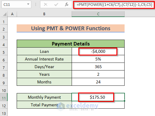
- At this time, press ENTER to see the amount of the Monthly Payment.
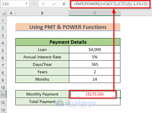
If I use the loan as negative then the result will be in black color. Which means the amount is credited. Besides, the red color denotes the amount as debit.
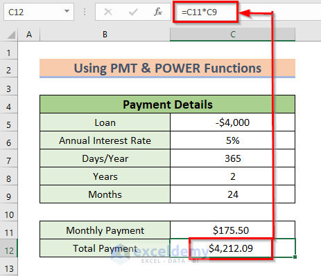
Furthermore, by multiplying the total months with the monthly payment, I will find out the total payment.
- Now, type the following formula in cell C12.
=C11*C9- Finally, press ENTER to see the amount of the Total Payment.
3. Using Generic Formula to Calculate Simple Interest Loan Payments in Excel
You can use the generic formula to calculate the total loan payment with simple interest and constant monthly payments.
Steps:
- Firstly, select a different cell C10 where you want to calculate the Total Payment.
- Secondly, use the corresponding formula in the C10 cell.
=C5*(1+C6*C7)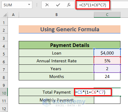
Formula Breakdown
- In this formula, I have multiplied Annual Interest Rate, C6 with Years, C7.
- After that, I have added 1.
- Furthermore, I have multiplied the whole result with the loan, C5.
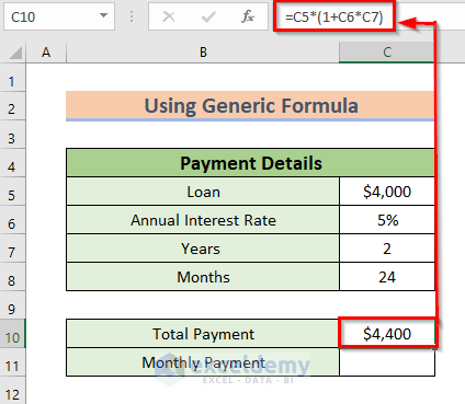
- At this time, press ENTER to see the amount of the Total Payment.
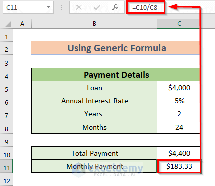
Subsequently, I will calculate the monthly payment by dividing the total payment by the total months.
- Firstly, select a different cell C11.
- Secondly, write the corresponding formula in the C11 cell.
=C10/C8- At this time, press ENTER to see the amount of the Monthly Payment.
Read More: How to Calculate Simple Interest on Reducing Balance in Excel
4. Inserting PV Function to Calculate Total Affordable Loan
You can use the PV function to calculate the total affordable loan.
Steps:
- Firstly, select a different cell C11 where you want to calculate the Affordable Loan.
- Secondly, use the corresponding formula in the C11 cell.
=PV(C7,C9,C5)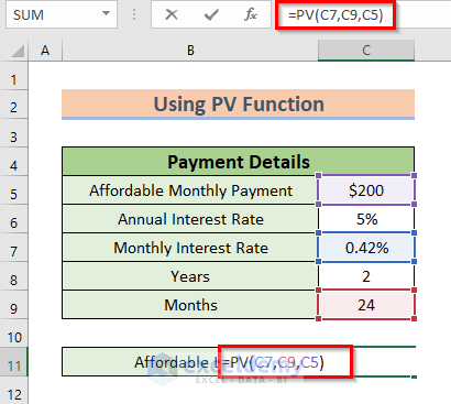
Formula Breakdown
In this formula, the PV function returns the present value of an investment.
- C7 denotes rate as the monthly interest rate.
- C9 denotes NPER as the total period of payment.
- C5 denotes PMT as the affordable monthly payment.
- Now, press the ENTER to get the affordable loan.

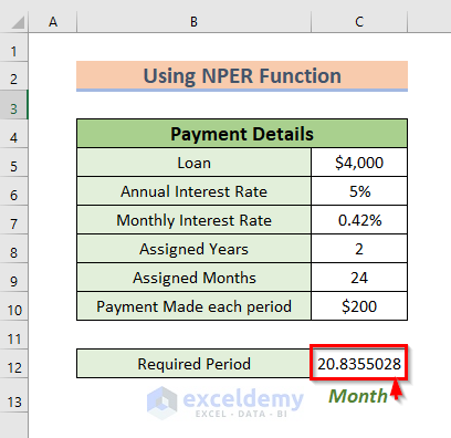
5. Using the NPER Function to Calculate Required Payment Period
You can employ the NPER function to calculate the required time period for paying the loan.
Steps:
- Firstly, I select the C12 cell for calculating the required period.
- Secondly, use the following formula in the C12 cell.
=NPER(C7,-C10,C5,,1)
Formula Breakdown
In this formula, the NPER function gives the required payment period as months.
- C7 denotes the monthly interest rate as rate.
- C10 denotes payment made in each period as PMT.
- C5 denotes the total loan as PV.
- 1 denotes the beginning of the period.
- Finally, press ENTER to get the result.
Practice Section
Now, you can do practice by yourself.

Download Practice Workbook
You can download the practice workbook from here:
Conclusion
I hope you found this article helpful. Here, I have explained 5 methods of how to calculate simple interest loan payments in Excel.
Please, drop comments, suggestions, or queries if you have any in the comment section below.
Related Articles
- How to Calculate Simple Interest and Compound Interest in Excel
- How to Calculate Daily Simple Interest in Excel
<< Go Back to Simple Interest Formula in Excel | Excel for Finance | Learn Excel
Get FREE Advanced Excel Exercises with Solutions!
