How to Calculate Simple Interest on Reducing Balance in Excel

Introduction to Simple Interest on Reducing Balance

There are two types of financial terms to pay the loan. The first one is Flat Rate Interest and another is Reducing the Balance Rate. Reducing the Balance Rate is a better approach when you are handling your loan. We will calculate the Reducing Rate of Interest using the above loan details.

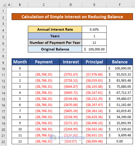
A loan of amount $100,000.00
Annual percentage rate (APR) 50%
Tenure of the Loan: 1 year
Payment Frequency: Monthly

If the Payment Frequency is monthly, we have to calculate the Rate for a month: Annual Percentage Rate / 12 = 0.00792

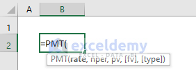
We also have to calculate the monthly PMT for the loan using Excel’s PMT function: =PMT(rate, nper, loan)

Here,

rate = 0.00792
nper = 12; [nper = number of total periods]
loan = -100,000

This returns the value: (8,768.35)

4 Quick Steps to Calculate Simple Interest on Reducing Balance in Excel

Let’s assume we have an Excel large worksheet that contains the information about the simple interest in the reducing balance. We will calculate the simple interest in reducing balance from our dataset using Excel’s PMT, IPMT, and PPMT financial formulas.

Step 1 – Use the PMT Function to Calculate Payment

The syntax of the function is,

=PMT(rate, nper, pv, [fv],[type])

Where the rate is the interest rate of the loan, nper is the total number of payments per loan, pv is the present value i.e. the total value of all the loan payments at present, [fv] is future value i.e. the cash balance one wants to have after the last payment is done, and [type] specifies when the payment is due.

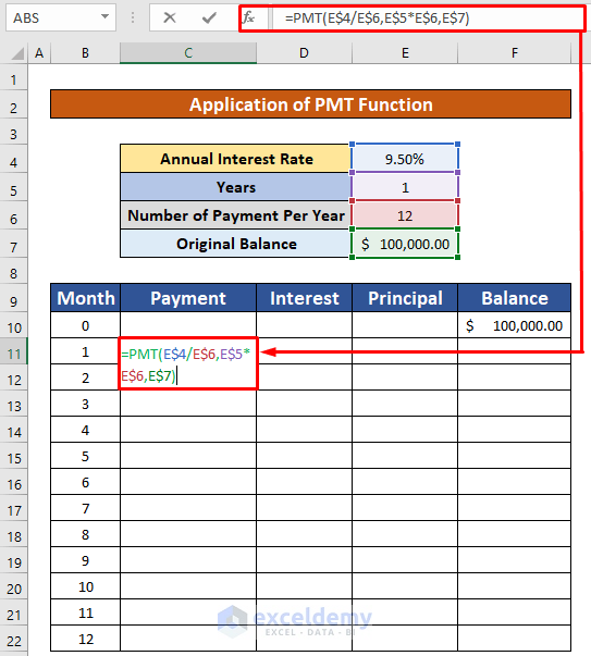
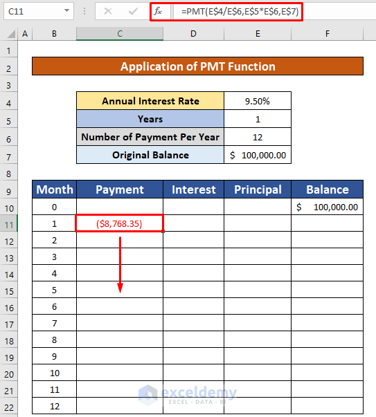
Select cell C11 and use the PMT function in that cell:

=PMT(E$4/E$6,E$5*E$6,E$7)

E$4 is the Annual Interest Rate, E$6 is the number of payments per year, E$5 is the number of years, and E$7 is the original price of the car. We use the dollar ($) sign for the absolute reference of a cell.

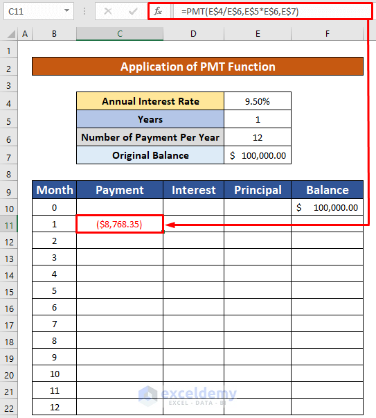
Press Enter. You will get the payment ($8,768.35) as the output of the PMT function.

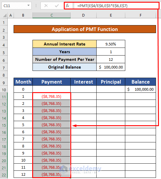
AutoFill the PMT function to the rest of the cells in column C.

You will be able to calculate the payment of the loan per month which has been given in the below screenshot.

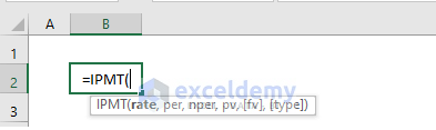
Step 2 – Apply the IPMT Function to Determine Interest of Payment

The syntax of the function is

=IPMT(rate, per, nper, pv, [fv],[type])

Where the rate is the interest rate per period, per is a specific period; must be between 1 and nper, nper is the total number of payment periods in a year, pv is the current value of a loan or investment, [fv]is the nper payments future worth, [type] is the payments behavior.

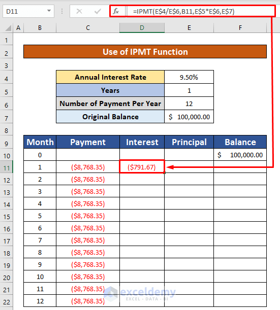
Select the cell D11 and use the IPMT function in the Formula Bar:

=IPMT(E$4/E$6,B11,E$5*E$6,E$7)

E$4 is the Annual Interest Rate, E$6 is the number of payments per year, B11 is the number of months, E$5 is the number of years, and E$7 is the original price of the car.

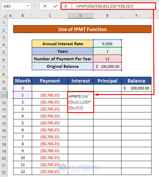
Press Enter. You will get the interest of payment ($791.67).

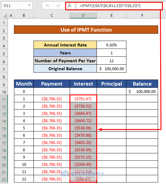
AutoFill the IPMT function to the rest of the cells in column D.

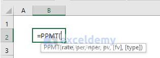
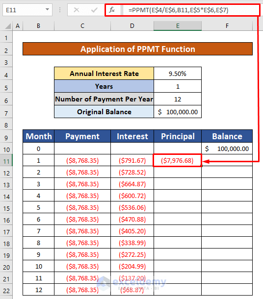
Step 3 – Insert the PPMT Function to Calculate Principal of Payment

The syntax of the function is,

=IPMT(rate, per, nper, pv, [fv],[type])

Where the rate is the interest rate per period, per is a specific period; must be between 1 and nper, nper is the total number of payment periods in a year, PV is the current value of a loan or investment, [fv]is the nper payments future worth, [type] is the payments behavior.

Select the cell E11 and type the PPMT function in the Formula Bar:

=PPMT(E$4/E$6,B11,E$5*E$6,E$7)

E$4 is the Annual Interest Rate, E$6 is the number of payments per year, B11 is the number of month, E$5 is the number of years, E$7 is the original price of the car.

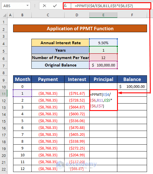
Press Enter.

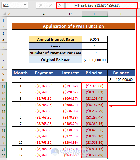
AutoFill the PPMT function to the rest of the cells in column E.

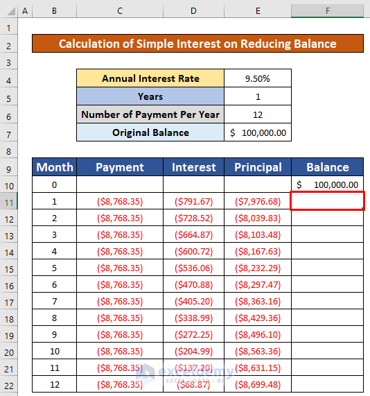
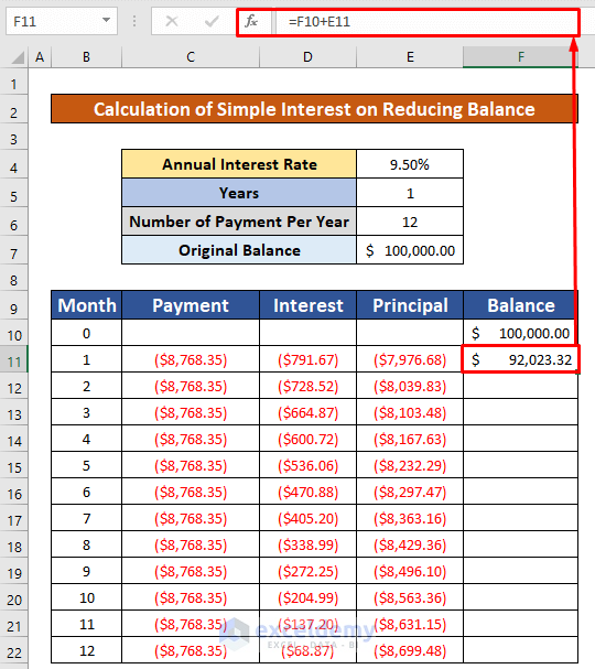
Step 4 – Use Mathematical Formula to Calculate Simple Interest on Reducing Balance

Select cell F11.

Use the following formula:

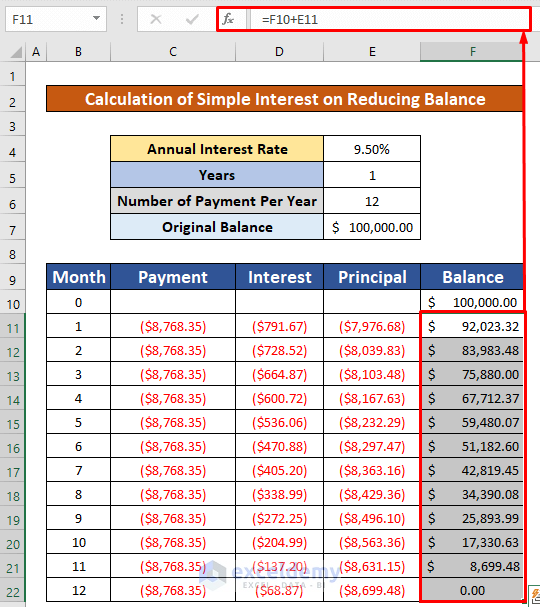
=F10+E11

F10 is the initial price of the car, and E11 is the total payment after the first month.

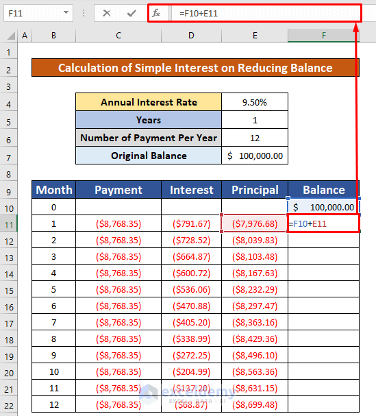
Press Enter.

AutoFill to the other cells in the column to determine when the balance will be reduced to 0.

Things to Remember

Each month, the loan debt is decreased as a result of the payments. The accumulated interest must decrease as the loan balance decreases.

#DIV/0 error occurs when the denominator is 0 or the reference of the cell is not valid.

The #NUM! error occurs when the per argument is less than 0 or is greater than the nper argument value.

Download the Practice Workbook

Calculation of Simple Interest on Reducing Balance.xlsx

<< Go Back to Simple Interest Formula in Excel | Excel for Finance | Learn Excel

Get FREE Advanced Excel Exercises with Solutions!

4 Comments

Alade Israel Mar 19, 2025 at 10:31 PM

Good day.

pls, what of if the loan is for 6month, how can someone calculate it using excel spreed sheet.

Thanks
- Reply
  Shamima Sultana Mar 20, 2025 at 11:12 AM
  
  Hello Alade Israel,
  
  If the loan is for 6 months, you can calculate the simple interest on a reducing balance in Excel by following these steps:
  
  Set up your columns: Create columns for Month, Beginning Balance, Interest, Principal Payment, and Ending Balance.
  Calculate Interest: Use the formula:
  
  =Beginning Balance * Interest Rate / 12
  (assuming the interest rate is annual).
  
  Calculate Principal Payment: If it’s an equal installment loan, subtract the interest from the monthly payment.
  Update the Ending Balance:
  =Beginning Balance – Principal Payment
  Drag the formulas down for the 6 months.
  
  Regards
  ExcelDemy
F.Snipes Apr 22, 2025 at 1:54 PM

Good day.

How should i calculate if the loan is for 5years with 8% interest rate per annum, how can i calculate it using excel spreed sheet.

Thanks
- Reply
  Shamima Sultana Apr 22, 2025 at 10:42 PM
  
  Hello F. Snipes,
  
  Thank you for your question! To calculate a 5-year loan with an 8% annual interest rate using Excel, you can use the PMT function for equal monthly payments or create a loan amortization schedule using the reducing balance method.
  
  Here’s a quick method using PMT:
  =PMT(8%/12, 5*12, -Loan_Amount)
  
  1. 8%/12 is the monthly interest rate.
  2. 5*12 is the total number of payments (months).
  3. Loan_Amount is the total loan you took (make sure it’s entered as a positive number).
  
  Regards
  ExcelDemy