Flat Rate Interest
Many people fail to understand these two financial terms: “flat rate interest” and “reducing balance rate”. This is the formula to calculate the flat rate of interest.
Flat Rate Interest = (Loan Amount x Number of Years x Annual Percentage Rate) / Total Number of Installments
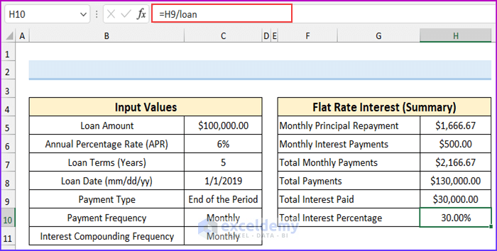
It is easier to understand this definition with an example. Suppose you took a loan for $100,000 with an annual percentage rate (APR) of 6%. You took the loan for 5 years and you have to pay monthly installments.. Your flat rate interest will be ($100,000 x 5 x 6%) / 60 or, $500. This is the interest that you will pay with every installment. Now, let’s calculate your principal repayments.
Principal Repayment = Loan Amount / Total Number of Installments
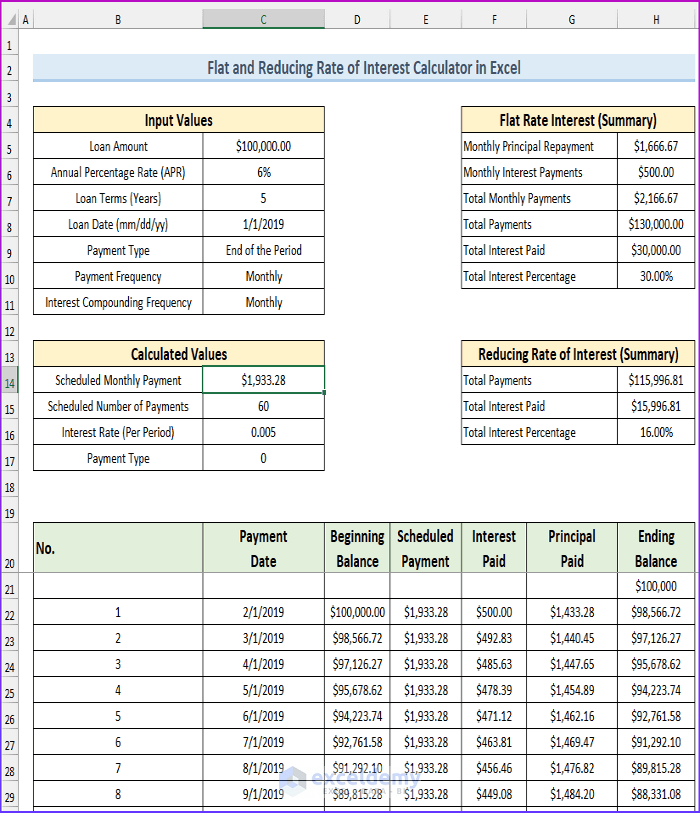
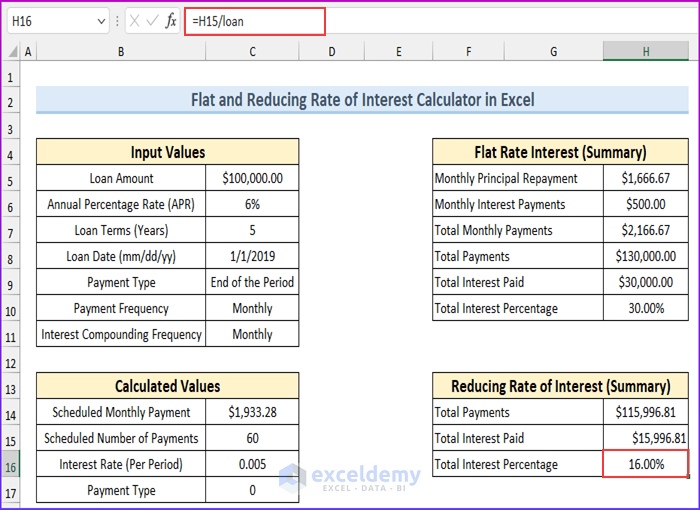
If we plug in the values it will be = $100,000 / 60 or $1,666.67. As such, your total monthly payment will be $500 + $1666.67 = $2166.67. You can see the summary of the above calculation (using my flat rate interest calculator) in the following image. The calculator also shows the following things:
- Total Payments: $130,000
- Total Interest Paid: $30,000
- You will 30% interest over the next 5 years.
The Reducing Rate of Interest
A reducing rate of interest is widely used by banks and financial institutions when you borrow money. We will calculate the reducing rate of interest using the below loan details.
- A loan of amount $100,000
- Annual percentage rate (APR) 6%
- Tenure of the Loan: 5 years.
- Payment Frequency: Monthly
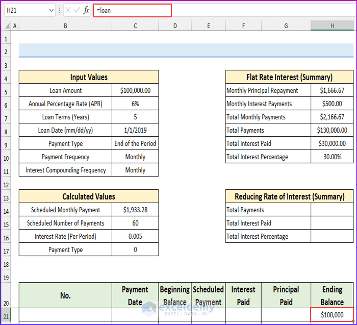
If the payment frequency is monthly, then first we have to calculate the rate for a month:
= Annual Percentage Rate / 12 = 6% / 12 or 0.005
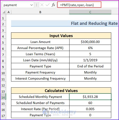
The next thing we have to calculate is the monthly PMT for the loan using Excel’s PMT function:
=PMT(rate, nper, -loan)
- Here, the values are:
- rate = 0.005
- nper = 60; [nper = number of total periods]
- -loan = -100,000; [loan is negative as we want the PMT to be a positive value].
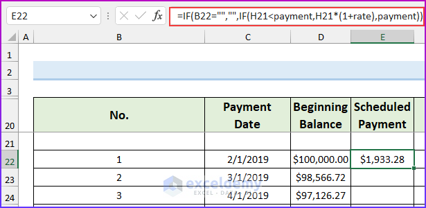
It returns a value of $1933.28.
Let’s discuss how the whole thing works:
1st Month:
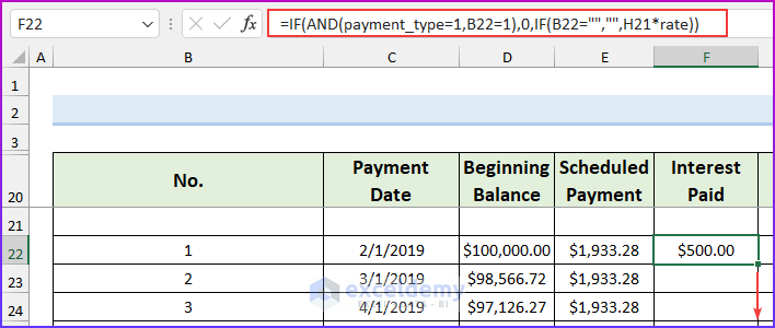
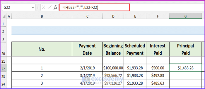
At the start of the first month, you have just taken the loan so the balance is $100,000. At the end of the first month, you’re paying $1933.28 (the PMT amount) to the financial institution. How much of this amount ($1933.28) is paid in interest? Your first month’s interest is: $100,000 x 0.005 = $500. This means $500 of $1933.28 is provided as the interest payment. The rest, $1933.28 – $500 = $1433.28, will be deducted from your principal. As a result, at the end of the first month, your new principal will be: $100,000 – $1433.28 = $98,566.72.
2nd Month:
At the start of the 2nd month, your new principal is: $98,566.72. At the end of the second month, you’re paying $1933.28 (the PMT amount) to the financial institution. How much of this amount ($1933.28) is paid in interest? Your second month’s interest is: $98566.72 x 0.005 = $492.83. The rest, $1933.28 – $492.83 = $1440.45, will be deducted from your principal. At the end of the second month, your new principal will be $98566.72 – $1440.45 = $97126.27. The whole process is visible in the following images.
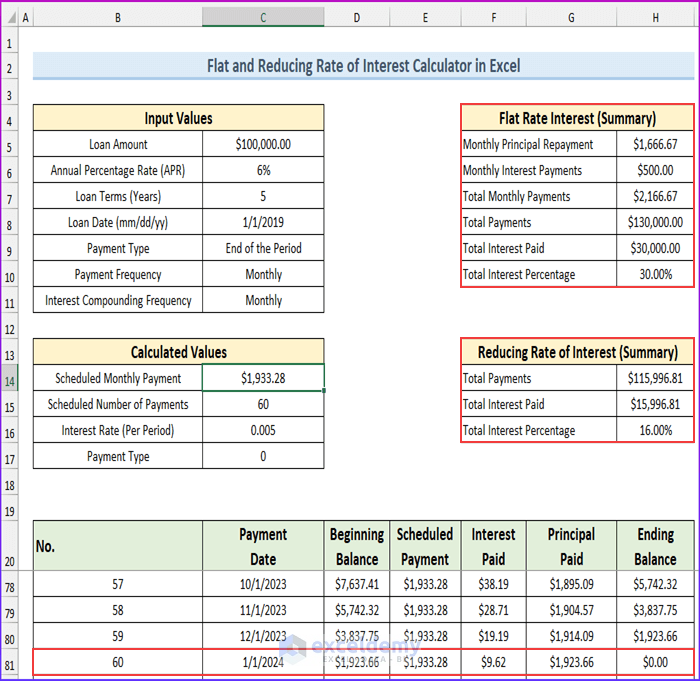
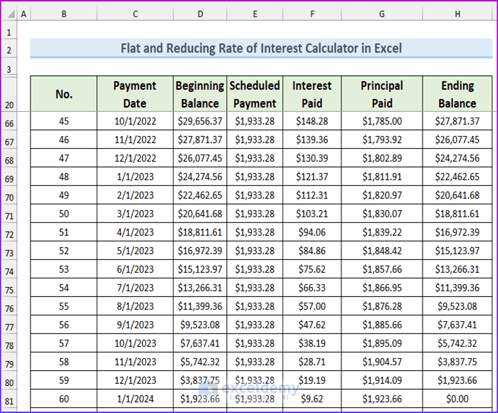
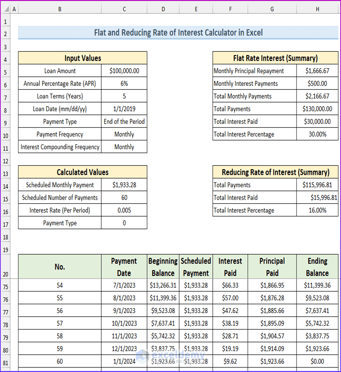
You see from the following image that with the last payment, we paid only $9.62 interest, and we cleared all our principal with the remaining amount of $1923.66. Our ending balance is $0.00. So that is our last payment to the financial institution.
The loan that uses the reducing rate of interest is simple. We only pay 16% interest overall in this system.
Step-by-Step Procedures to Create Flat and Reducing Rate of Interest Calculator in Excel
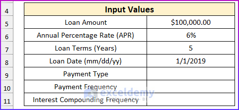
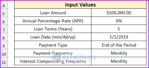
Step 1- Enter Required Values
- Input these values.
- Select cell C9.
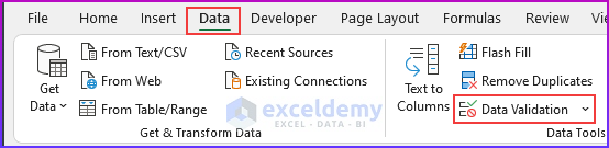
- From the Data tab, select Data Validation.
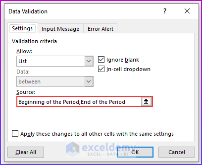
- Enter these values in the source field, separating them with a comma, and press OK.
- Beginning of the Period
- End of the Period
- The values for the payment frequency and interest compounding frequency are as follows. Enter these values inside the data validation source, separating each value with a comma.
- Weekly
- Bi-weekly
- Semi-monthly
- Monthly
- Bi-monthly
- Quarterly
- Semi-annually
- Yearly
Step 2 – Find Flat Rate Interest
We have used a table for the lookup range using the VLOOKUP function. This table is hidden to keep the users from changing the values by accident.
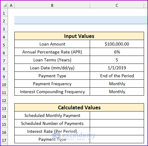
- Copy the information in the cell range B13:B17 into the corresponding fields.
- Enter this formula in cell C15.
=C7*VLOOKUP(payment_frequency,periodic_table,3,FALSE)
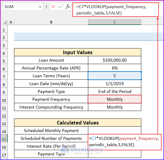
Formula Breakdown
- The payment_frequency is “Monthly”.
- The periodic_table is the lookup range for our function. We can see the table from the name range or by unhiding the “Tables” sheet.
- We will return values from the third column.
- We have used FALSE to indicate exact matching, and we are multiplying the data by the loan terms (years) value to get the value of the scheduled number of payments.
- From the Formulas tab, select Name Manager.
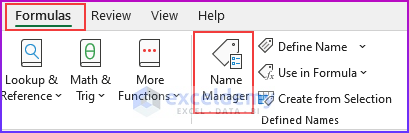
- A dialog box will pop up that will enable us to see the values of the named ranges.
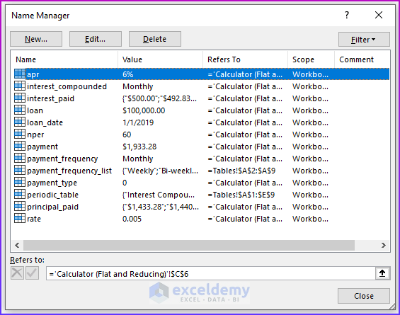
- We can unhide the “Tables” sheet to see the “periodic_table”.
- Enter this formula in cell C16:
=(1+apr/VLOOKUP(interest_compounded,periodic_table,3,0))^(VLOOKUP(interest_compounded,periodic_table,3,0)/VLOOKUP(payment_frequency,periodic_table,3,0))-1
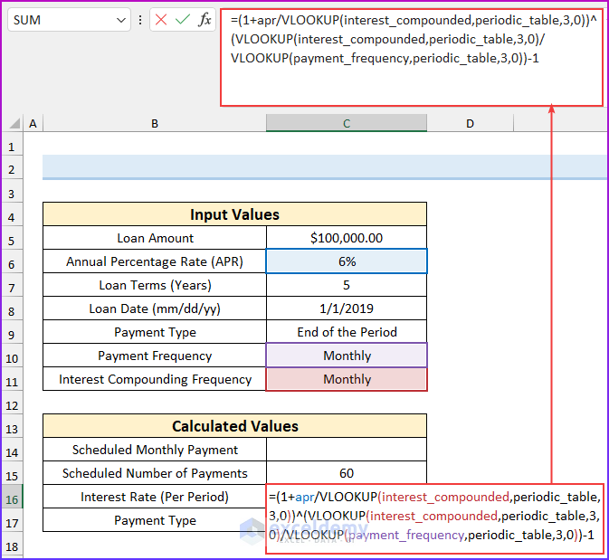
Formula Breakdown
- Here we have three VLOOKUP functions. Again, we have used the name range. “Interest_compunded” is in cell C11 and the value of “payment_frequency” is in cell C10.
- VLOOKUP(interest_compounded,periodic_table,3,0)
- Output: 12.
- VLOOKUP(payment_frequency,periodic_table,3,0)
- Output: 12.
- The formula reduces to, (1+apr/12)^(12)/12)-1
- Output: 0.00499999999999989.
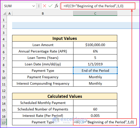
- Enter another formula in cell C17. We are using a conditional here. When the payment type is the beginning of the period, then the formula will return 1. Otherwise, we will get 0.
=IF(C9="Beginning of the Period",1,0)
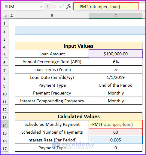
- Enter this formula and press ENTER. Using this formula, we can find the monthly installment.
=PMT(rate,nper,-loan)
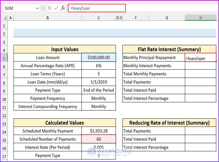
- To find the values of the flat rate of interest (summary), input this formula and press ENTER.
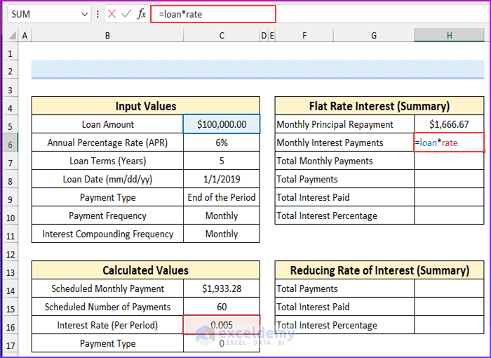
=loan/nper
- Input this formula and press ENTER.
=loan*rate
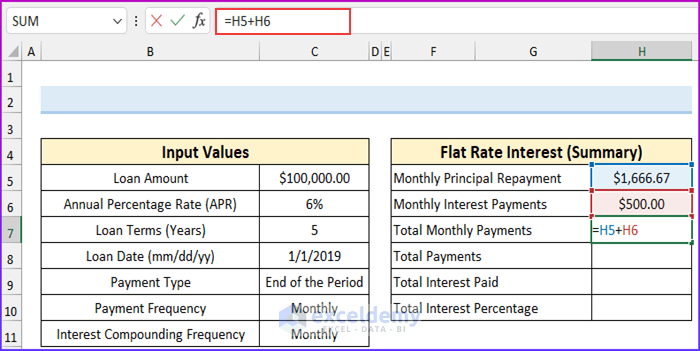
- Input this formula and press ENTER.
=H5+H6
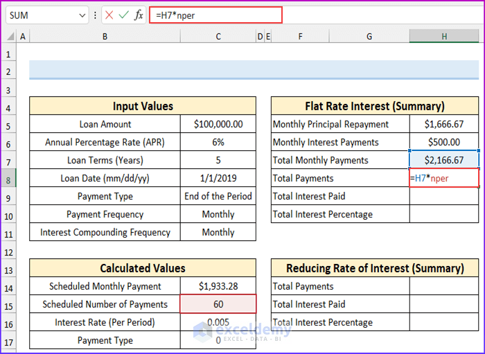
- Add this formula and press ENTER.
=H7*nper
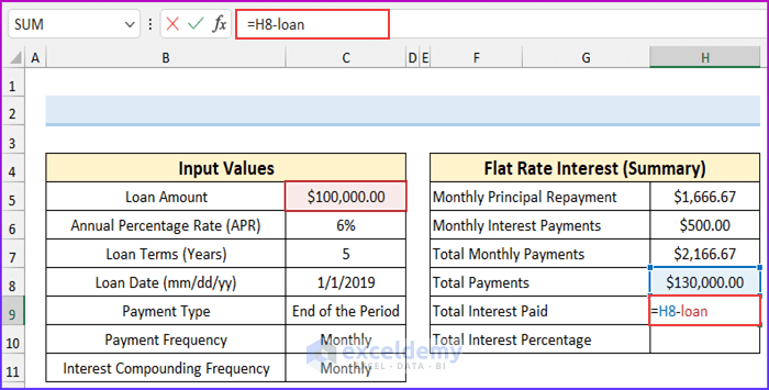
- Input this formula and press ENTER.
=H8-loan
- Add this formula and press ENTER.
=H9/loan
Read More: How to Perform Interest Rate Swap Calculation in Excel
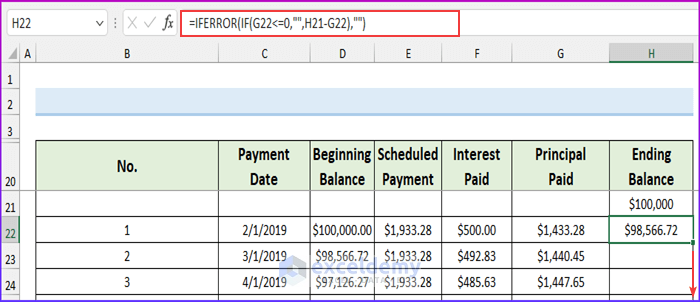
Step 3 – Calculate Payment Schedule
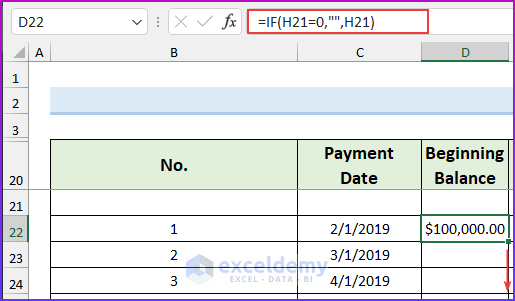
- Add the following formula to cell H21 and press ENTER.
=loan
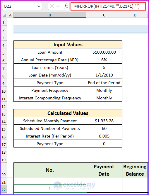
- Enter the following formula and drag the fill handle to all other cells you want to populate.
=IFERROR(IF(H21<=0,"",B21+1),"")
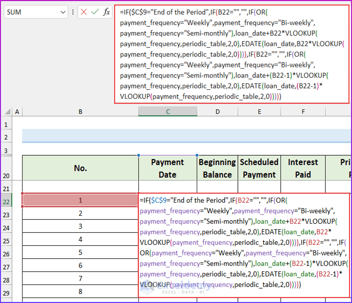
- Enter the following formula and drag the fill handle to all other cells you want to populate.
=IF($C$9="End of the Period",IF(B22="","",IF(OR(payment_frequency="Weekly",payment_frequency="Bi-weekly",payment_frequency="Semi-monthly"),loan_date+B22*VLOOKUP(payment_frequency,periodic_table,2,0),EDATE(loan_date,B22*VLOOKUP(payment_frequency,periodic_table,2,0)))),IF(B22="","",IF(OR(payment_frequency="Weekly",payment_frequency="Bi-weekly",payment_frequency="Semi-monthly"),loan_date+(B22-1)*VLOOKUP(payment_frequency,periodic_table,2,0),EDATE(loan_date,(B22-1)*VLOOKUP(payment_frequency,periodic_table,2,0)))))
Formula Breakdown
- We are using the nested IF formula.
- OR(payment_frequency=”Weekly”,payment_frequency=”Bi-weekly”,payment_frequency=”Semi-monthly”)
- Output: FALSE.
- loan_date+B22*VLOOKUP(payment_frequency,periodic_table,2,0)
- Output: 43467.
- EDATE(loan_date,B22*VLOOKUP(payment_frequency,periodic_table,2,0))
- Output: 43497.
- loan_date+(B22-1)*VLOOKUP(payment_frequency,periodic_table,2,0)
- Output: 43466.
- EDATE(loan_date,(B22-1)*VLOOKUP(payment_frequency,periodic_table,2,0))
- Output: 43466.
- Then, the formula reduces to, IF($C$9=”End of the Period”,IF(B22=””,””,IF(FALSE,43467,43497)),IF(B22=””,””,IF(FALSE,43466,43466)))
- Output: 43497.
- The actual value in cell C9 is “End of the Period”, therefore, the function will return true. Now, cell B22 is not blank. So, IF(FALSE,43467,43497) this part will be executed. As the logical condition is false, we will get the value 43497.
- Input this formula and use Drag Handle to autofill all other cells as required.
=IF(H21=0,"",H21)
- Enter the following formula and drag the fill handle to all other cells you want to populate.
=IF(B22="","",IF(H21<payment,H21*(1+rate),payment))
- Enter the following formula and drag the fill handle to all other cells you want to populate. If the payment type is at the beginning of the month and the value of cell B22 is 1, then it will return 0. Otherwise, it will return the “H21*rate” part.
=IF(AND(payment_type=1,B22=1),0,IF(B22="","",H21*rate))
- Enter the following formula and drag the fill handle to all other cells you want to populate.
=IF(B22="","",E22-F22)
- Enter the following formula and drag the fill handle to all other cells you want to populate.
=IFERROR(IF(G22<=0,"",H21-G22),"")
- The payment schedule will look like this.
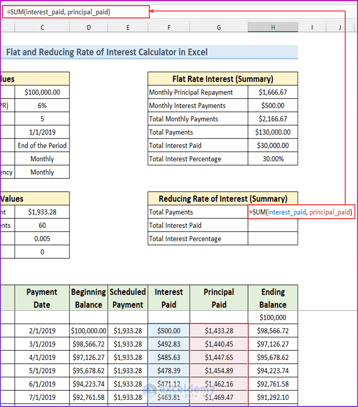
Step 4 – Calculate the Reducing Rate of Interest
We have named the cell range F22:F10971 and G22:G10971 as the interest_paid and principal_paid respectively.
- Enter the following formula.
=SUM(interest_paid, principal_paid)
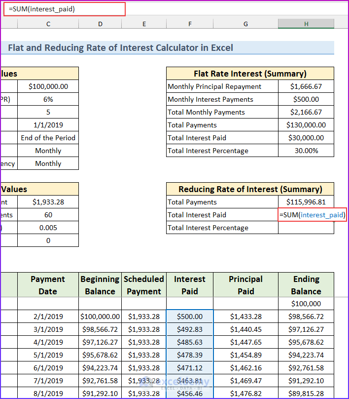
- Input this formula.
=SUM(interest_paid)
- Input the following formula and press ENTER.
=H15/loan
Instructions for Using This Calculator
Enter the following values to use this calculator:
- Loan Amount
- Annual Percentage Rate (APR)
- Loan terms (Years)
- Loan Date (mm/dd/yy)
- Payment type. This is a drop-down list. You will get two types of payments. End of the Period and Beginning of the Period. Choose the one that suits your loan.
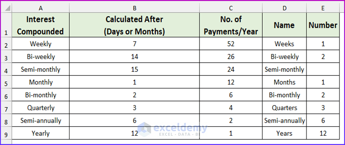
- Payment frequency: This is also a drop-down list. You can choose payment frequencies:
| Interest Compounded | Calculated After
(Days or Months) |
No. of Payments/Year |
|---|---|---|
| Weekly | 7 Days | 52 |
| Bi-weekly | 14 Days | 26 |
| Semi-monthly | 15 Days | 24 |
| Monthly | 1 Month | 12 |
| Bi-monthly | 2 Months | 6 |
| Quarterly | 3 Months | 4 |
| Semi-annually | 6 Months | 2 |
| Yearly | 12 Months | 1 |
- Interest Compounding Frequency: In most cases, your Payment frequency will be equal to Interest Compounding Frequency. In some countries, like Canada, interest is compounded semi-annually but payments are monthly. So, except in rare cases, your Payment frequency will always be equal to Interest Compounding Frequency.
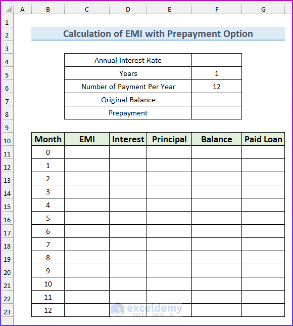
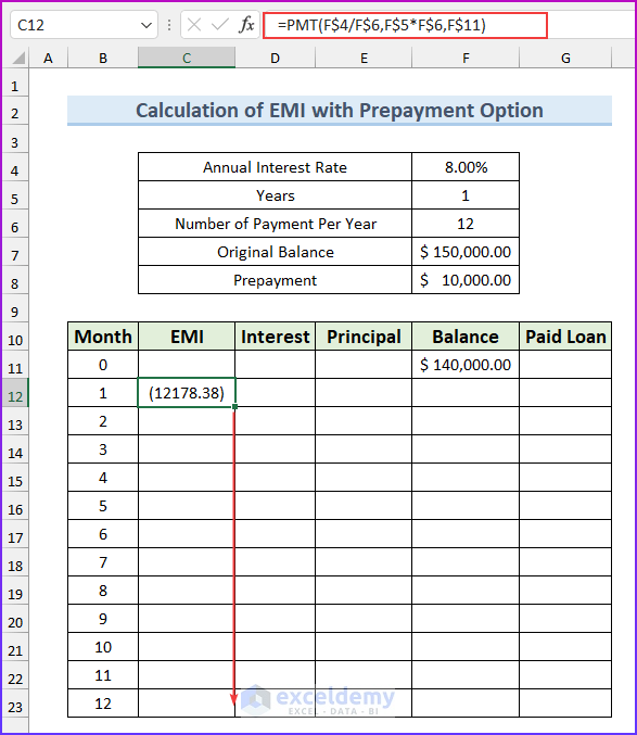
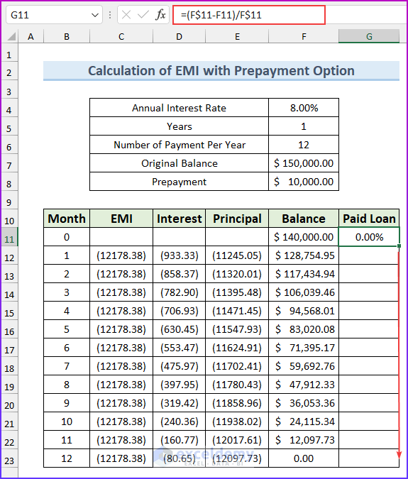
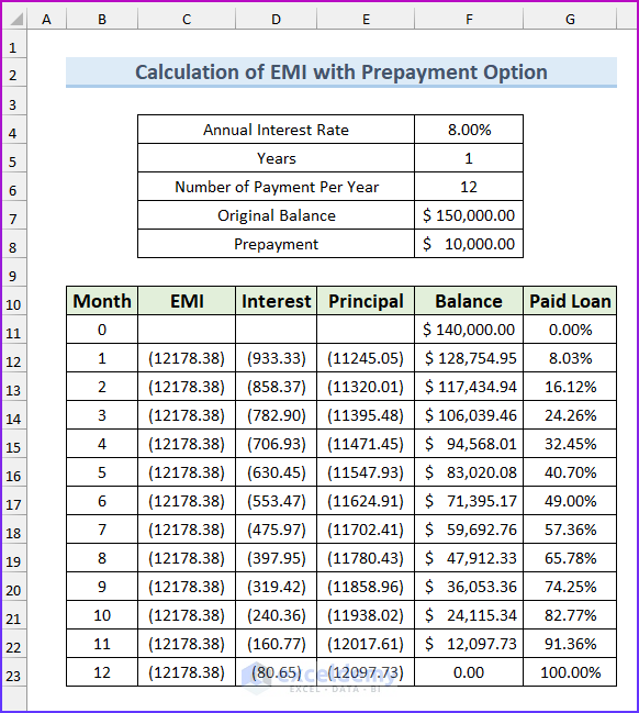
EMI Calculator with Prepayment Option in Excel Sheet
Let’s assume we have an Excel worksheet that contains the information about the EMI calculation with the prepayment option. We will calculate the EMI with the prepayment option from our dataset using Excel’s PMT and IPMT financial formulas. PMT stands for payment, and IPMT is used to get the interest on a payment.
Steps:
- Enter the information in all these fields. Our values are for one year, so we have created the template for 12 months. You can add more as needed.
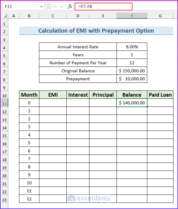
- Enter this formula to get the value of the beginning balance.
=F7-F8
- Input the following formula to return the value of EMI and use the Drag Handle to AutoFill all other cells as required.
=PMT(F$4/F$6,F$5*F$6,F$11)
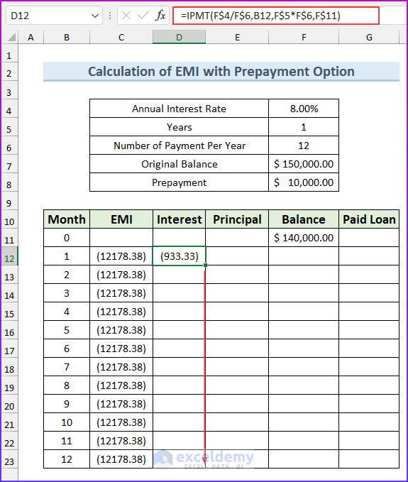
- Enter the following formula and drag the fill handle to all other cells you want to populate.
=IPMT(F$4/F$6,B12,F$5*F$6,F$11)
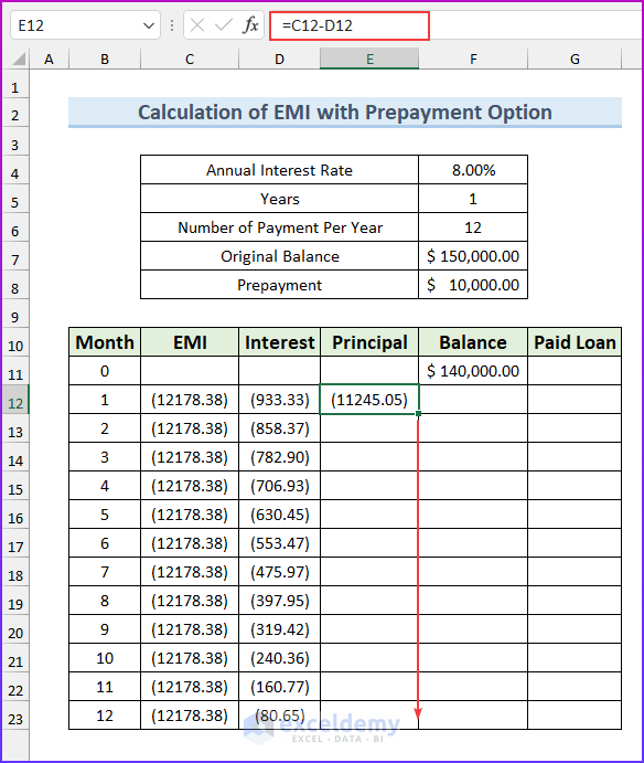
- Enter the following formula to get the principal amount and drag the fill handle to all other cells you want to populate.
=C12-D12
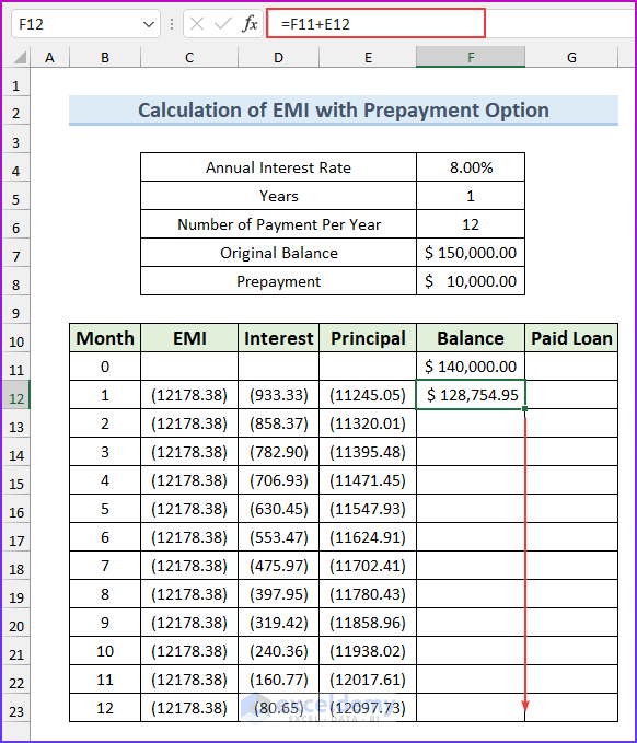
- Enter this formula to get the balance amount and drag the fill handle to all other cells you want to populate.
=F11+E12
- Enter this formula to get the percentage of loan paid and drag the fill handle to all other cells you want to populate.
=(F$11-F11)/F$11
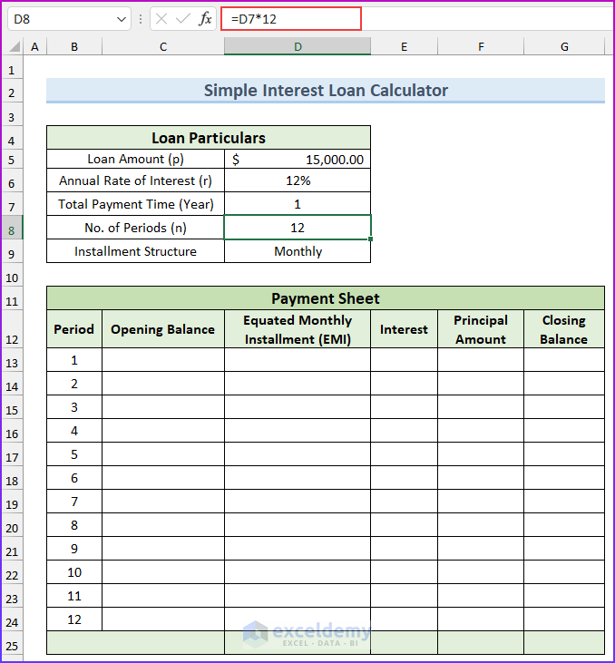
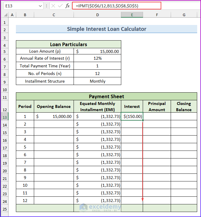
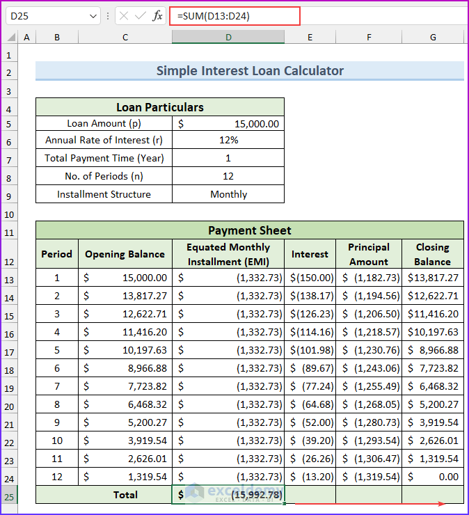
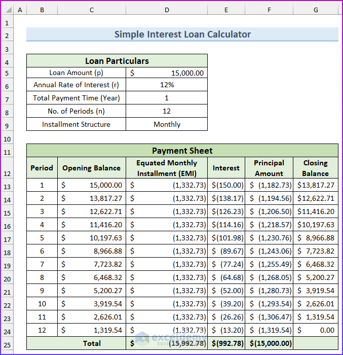
Simple Interest Loan Calculator Using Formula in Excel
Simple interest denotes the amount estimated from the principal amount of any loan taken from a bank or the initial contribution of any bank’s savings account. The mathematical expression of simple interest is:
I = P × R × n
Here the symbols denote the following things:
- I = The amount of earned interest from the principal amount.
- P = Principal amount
- R = Annual rate of interest
- n = Number of period
Steps:
- Enter the information in the following fields and add the following formula to cell D8.
=D7*12
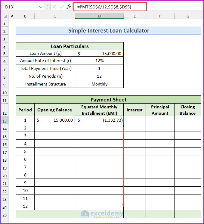
- Enter the following formula and drag the fill handle to all other cells you want to populate.
=PMT($D$6/12,$D$8,$D$5)
- Enter the following formula and drag the fill handle to all other cells you want to populate.
=IPMT($D$6/12,B13,$D$8,$D$5)
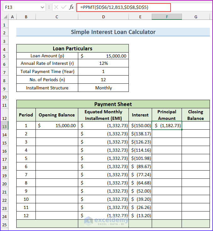
- Enter this formula in cell F13.
=PPMT($D$6/12,B13,$D$8,$D$5)
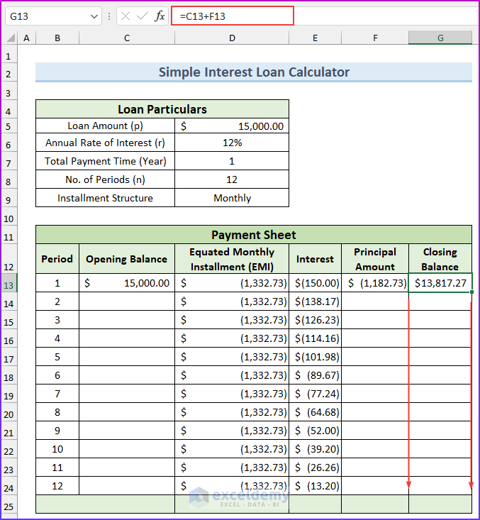
- Enter this formula to get the closing balance and fill in the formulas from columns F and G.
=C13+F13
- Enter the following formula and drag the fill handle to all other cells you want to populate.
=G13
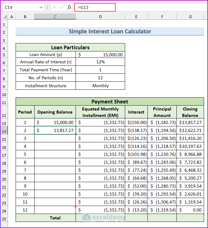
- Input this formula to get the total values and use the Drag Tool to the right to complete the rest of the row.
=SUM(D13:D24)
Download Practice Workbook
You can download the Excel file from the link below.
Related Articles
- How to Perform Interest Rate Sensitivity Analysis in Excel
- How to Calculate Effective Interest Rate On Bonds Using Excel
<< Go Back to Interest Rate Calculator | Finance Template | Excel Templates
Get FREE Advanced Excel Exercises with Solutions!

such a great help in my work since i handled loan applications. how about the pro-rata interest ? example the loan is granted on the 10th of the month. how do i include in the calculator the pro-rata interest. the payment is always at the end of the month so how do i include the pro-rata days to include in the monthly payment
Hi Lisa. You can use the YEARFRAC function to calculate the days difference in fraction of that year. Then, you can multiply the result with the annual interest payment (in this case, scheduled monthly payment*12) to include the pro-rata interest.
hello myself ravneet from patiala i want to know which is best for small finance bank (jivan etc)
1st and last installment change other remain same send formala detail for excel to find out
Hello Ravneet, you can follow this article and adjust your payments on the “Extra Payment” column.
Hi,
Have gone through the template and found it quite interesting and will score it 8 out 10 reason:
1. On Web most of the experts had shared template and urs is having same feasible solution. But have given two addition points in 8 belongs to combine approach of Straight line and reducing Method.
2. ‘ve hold 2 points for one unique reason, suppose Mr. X had taken loan of USD 150000 for 5 Years at 18% intt. rate and at the end of 23rd installment he paid USD 60000 than in that particular scenario template got failed.
Hoping that you got my point.
Thank you sir such a great work in financial tools for finance related
You’re most welcome, Sumit!
Hi, I m trying to learn how to use excel sheets. The one thing I really need but have not figured out is this.
I want to be able to put in a fixed value, that is changed with a set interest rate monthly, and able to auto calculate the new balance over a set number of months. The interest rate needs to be where it can be either a positive or negative value. could you share a formula that excel could use for this purpose?
What if I have a fixed payment schedule? How do I handle interest calculations around that?
THAT WAS GREAT HELP FOR ME
Congratulations the loan calculator is good, but try to adjust the loan term(year), some are borrowing in short terms like 1month, 3months or 10months.Therefore put the loan term in months also.
Thank you!
Very helpful indeed, makes my work so easy… thank you very much sir…
Best regards, Mario!
I do love this template, thank you for your effort
my only comment is the template doesn’t consider if there is a grace period. i tried to change the date of the first installment as i thought it considers Today date and the first installment but it doesn’t.
Thanks you
Mostafa
Different credit cards have different grace periods. You can send us your Excel file and we will look into it.
Pls advise if the interest rate is floating and revised every quarter basis LIBOR then for a given period of time how do we calculate the reducing rate of interest equivalent to the variable interest rate.
You can split the payment schedule into desired quarters and calculate the payments using that quarters’ interest rates.
Thank you so much making it easy for me to understand my actual costing.
Thank you so much for making a clear and concise explanation of this concept. THUMBS UP!!!
Excellent..
Dear Sir
Can be available Loan Amortization table in excel
Can it be possible client wise auto update loan amortization table?
Also if possible interest rate change so auto update automatic in excel
Extra Payments means(Start at Payment No,Extra Payment,Payment Interval,Extra Annual Payment,Payment,Total Extra Payments)
Additional Payment,
Variable or Fixed Rate ,
Impact of interest rate HIKE on your loan EMI & repayment schedule & Impact of interest rate CUT on your loan EMI & repayment schedule ?
how to create in excel & Suppose provide only interest
Hello BHAVNESH,
Have a look at Article 1 and Article 2. I hope it will help you to meet your desire.