The term Tiered Interest Rate means that, according to the policy of the specific country, different ranges of values attract different rates of interest. In this article, we will describe how to use a tiered interest rate calculator in Excel with 3 useful examples.
To apply a tiered interest rate, we need the range of amounts with different interest rates. Each will create a single tier. When an account balance is provided, we will check which tier it falls under and return the value of the tiered interest.
Example 1 – Using SUMPRODUCT Function on the Current Account Balance
The SUMPRODUCT function can single-handedly calculate the tiered interest rate.
Steps:
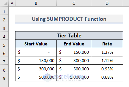
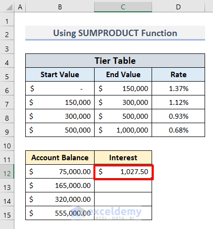
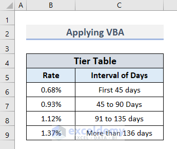
- Create a Tier Table according to your local conditions like this:
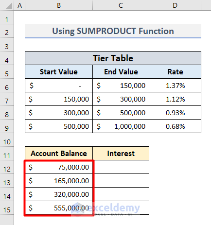
- Create another table with headings Account Balance and Interest.
- Insert the amounts in different accounts in the range B12:B15.
- Enter the following formula in cell C12:
=SUMPRODUCT((B12<=$C$6:$C$9)*(B12>$B$6:$B$9)*(B12-$B$6:$B$9)*$D$6:$D$9)+SUMPRODUCT(((B12>$C$6:$C$9)*($C$6:$C$9-$B$6:$B$9))*$D$6:$D$9)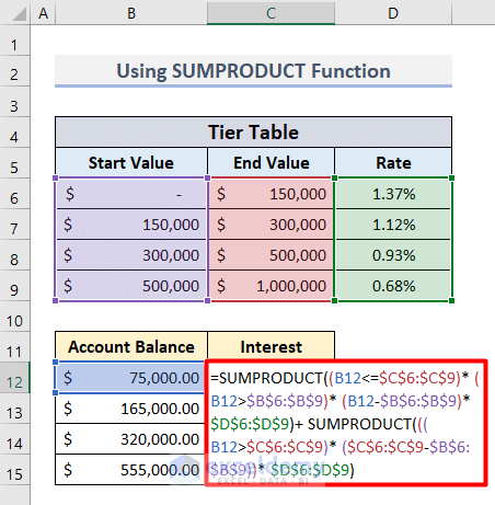
- Press Enter to return the first Tiered Interest Rate.
How Does the Formula Work?
- In this formula, there are 2 SUMPRODUCT functions.
- The first one is used to calculate whether the balance in cell B12 is above or below the values in tiers B6:B9 and C6:C9. It also calculates the corresponding percentage from D6:D9.
- The second SUMPRODUCT function returns the value that matched the tier level and corresponding percentages.
- Then the formula adds both numbers and returns the final interest rate.
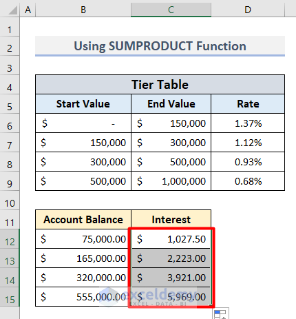
- Use the AutoFill tool to get all the Interest values for each Account Balance.
Read More: How to Convert Monthly Interest Rate to Annual in Excel
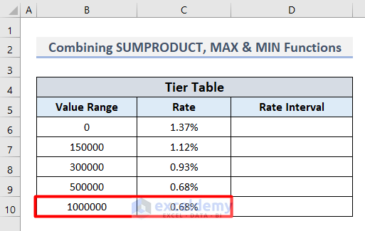
Example 2 – Combining SUMPRODUCT, MAX & MIN Functions for a More Dynamic Application
Steps:
- Insert a new tier that assigns values over 1000000 an interest rate of 0.68%.
- In cell D6, insert this formula to get the first Rate Interval:
=C6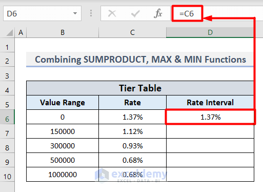
- Apply this formula in cell D7 to return the second Rate Interval in the Tier Table.
=C7-C6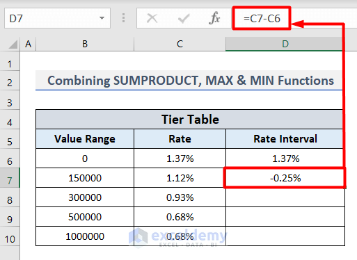
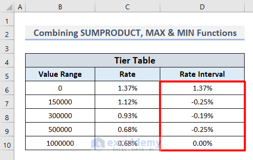
- Apply AutoFill to return all the values like this:
- Insert this formula in cell C13:
=SUMPRODUCT((MIN(B13,MAX($B$6:$B$10))-$B$6:$B$10)*$D$6:$D$10*((MIN(B13,MAX($B$6:$B$10))-$B$6:$B$10)>=0))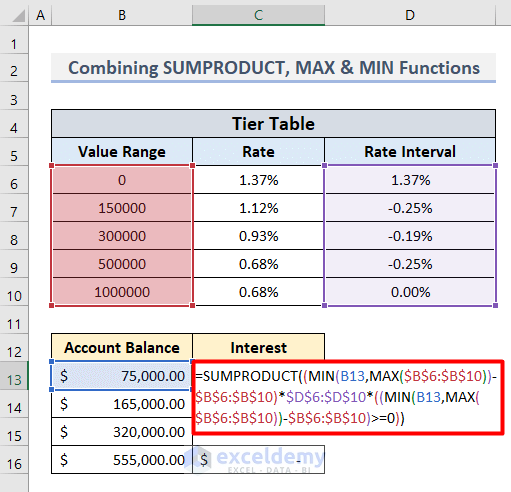
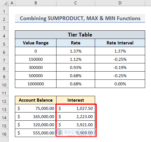
- Press Enter and AutoFill to get all the Interest Rates at once.
Read More: How to Use Nominal Interest Rate Formula in Excel
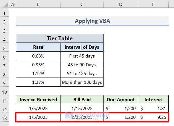
Example 3 – Using Excel VBA
Now let’s calculate the Tiered Interest Rate based on dates and due amounts. This process is very effective for keeping day-to-day records. Consider the following conditions in the Tier Table:
Steps:
- Create a new table with the titles Invoice Received, Bill Paid, Due Amount and Interest.
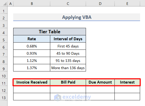
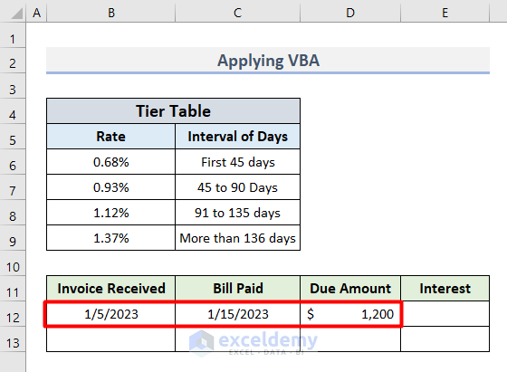
- Insert the initial values according to your requirement as shown below.
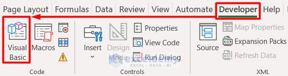
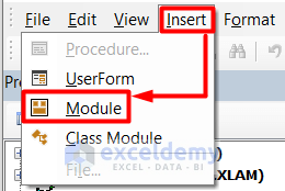
- Select Visual Basic under the Code group from the Developer tab.
- Choose Module from the Insert tab in the Microsoft Visual Basic for Applications window.
- Insert this code in the Code window:
Function TieredInterest(Inv As Date, Bill As Date, DueAmt As Double)
Dim Lt As Long
Lt = Bill - Inv
Const Tier0 = 0.0068     '-- First 45 Days
Const Tier1 = 0.0093 '-- 46 to 90 Days
Const Tier2 = 0.0112   '-- 91 to 135 Days
Const Tier3 = 0.0137 '-- 136+ days
Select Case Late
Case 0 To 45: TieredInterest = Round(Tier0 * DueAmt * (Lt / 45), 2)
Case 46 To 90: TieredInterest = Round(Tier1 * DueAmt * ((Lt - 45) / 45), 2)
Case 91 To 135: TieredInterest = Round(Tier1 * DueAmt * (45 / 45), 2) + Round(Tier2 * DueAmt * ((Lt - 90) / 45), 2)
Case 136 To 10000: TieredInterest = Round(Tier1 * DueAmt * (45 / 45), 2) + Round(Tier2 * DueAmt * (45 / 45), 2) + Round(Tier3 * DueAmt * ((Lt - 135) / 45), 2)
End Select
End Function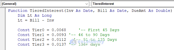
- Press Ctrl + S to save the code and close the window.
- Insert this formula in cell E12 to get the Interest value for the given Due Amount dated within 45 days.
=TiredInterest(B12,C12,D12)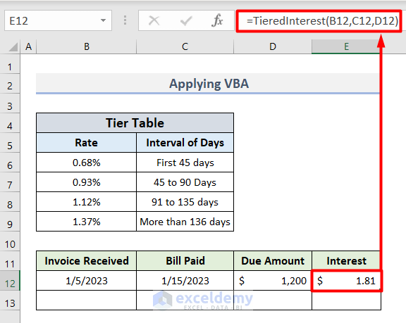
- Provide dates greater than 45 days to return the Interest based on the Tier Table.
Download Practice Workbook
Related Articles
- Perform Interest Rate Sensitivity Analysis in Excel
- How to Perform Interest Rate Swap Calculation in Excel
- Calculate Weighted Average Interest Rate in Excel
- How to Calculate Interest Rate from EMI in Excel
- Loan Amortization Schedule with Variable Interest Rate in Excel

