How to Calculate the Weighted Average Interest Rate in Excel

The Weighted Average Interest Rate

The Weighted Average Interest Rate refers to an average that is adjusted to show the impact of each loan on total debt.

Formula to Calculate the Weighted Average Interest Rate

A₁, A₂, and A_n are the Loan Balances.
i₁, i₂, and i_n are the Interest Rates.

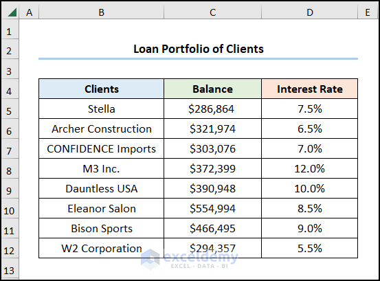
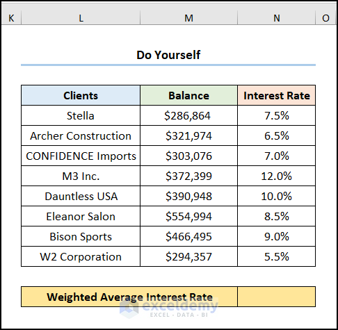
The Loan Portfolio of Clients dataset contains “Clients”, “Balance”, and “Interest Rate”.

Method 1 – Using an Arithmetic Formula

Steps:

Go to the D14 >> enter the formula below >> press ENTER.

=(C5*D5+C6*D6+C7*D7+C8*D8+C9*D9+C10*D10+C11*D11+C12*D12)/(C5+C6+C7+C8+C9+C10+C11+C12)

The product of the “Balance” and “Interest Rates” columns was calculated and divided by the total “Balance”.

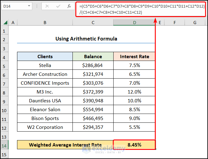
This is the output.

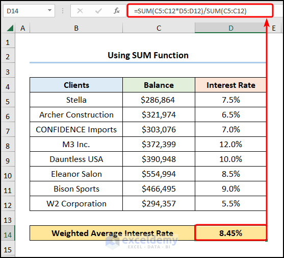
Method 2 – Utilizing the SUM Function

Steps:

Go to D14 >> enter the expression below >> press ENTER.

=SUM(C5:C12*D5:D12)/SUM(C5:C12)

C5:C12 and D5:D12 arrays represent the “Balance” and “Interest Rate” columns.

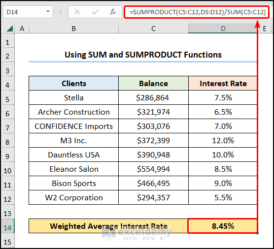
Method 3 – Applying the SUMPRODUCT and the SUM Functions

Steps:

Enter the formula in D14 >> press ENTER.

=SUMPRODUCT(C5:C12,D5:D12)/SUM(C5:C12)

Formula Breakdown

SUM(C5:C12) → adds all numbers in a range of cells. Here, the values in C5:C12.
- Output → $2,991,107
SUMPRODUCT(C5:C12,D5:D12) → returns the sum of the products of the “Balance” and “Interest Rate” arrays. Here, C5:C12 and D5:D12 are array1 and array2 arguments in which the values of columns C and D are multiplied.
- Output → 252789.785
SUMPRODUCT(C5:C12,D5:D12)/SUM(C5:C12) → becomes
- $2,991,107 / 252789.785 → 8.45

Note: Open the Format Cells dialog box by pressing CTRL + 1 and change the cell formatting to percentage.

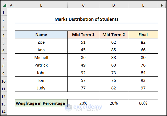
How to Calculate the Weighted Average with Percentages in Excel

The dataset showcases students’ “Name”, “Mid Term 1”, “Mid Term 2” and “Final” marks. Exam values in B13:E13 are in percentage.

Steps:

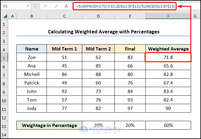
Enter the formula into F5 >> press ENTER >> drag the Fill Handle to copy the formula to the cells below.

=SUMPRODUCT(C5:E5,$D$13:$F$13)/SUM($D$13:$F$13)

C5:E5 points to the marks scored by “Zoe”, whereas D13:F13 indicates the “Weightage in Percentage”. The SUMPRODUCT function yields the summation of the products of the marks scored in“Mid Term 1”, “Mid Term 2” and “Final” exams and their “Weightage in Percentage” values.

Note: Use Absolute Cell Reference by pressing the F4.