How to Create an Effective Interest Method of Amortization in Excel – 2 Examples

Overview of Effective Interest Method of Amortization

An amortizing loan is a loan in which the principal is paid throughout the life of the loan, according to an amortization plan.

Consider the following situation:  the total value of a car is $200000.00, the annual interest rate is 10%, and you will pay the loan within 1 year. The Loan Amortization Schedule shows periodic payments, the number of years left to repay the loan, how much you owe, how much interest you are paying, and the initial amount owed.

The effective interest method of amortization is the percentage of interest or financial product if compound interest amasses over a year with no payments. It is the true interest rate on a loan. Usually, a frequent compounding period results in a higher compounding rate.

Example 1 – Effective Interest Method of Amortization for Bonds Sold on Discount

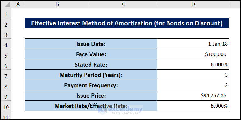
These are the details:

Issue Date: 1st Jan 2018

Face Value: $100,000

Stated Rate/Nominal Rate/Coupon Rate/APR: 6%

Market Rate / Effective Annual Interest Rate: 8%

Maturity Period: 3 years

Interest Payment Frequency: Semi-annually

Issue Price: $94,757.86 (the bond is selling at a discount)

Calculate the effective interest method of amortization for the bond sold on discount:

Step 1: Enter Values in the Journal

Record the transactions on 1st Jan 2018.

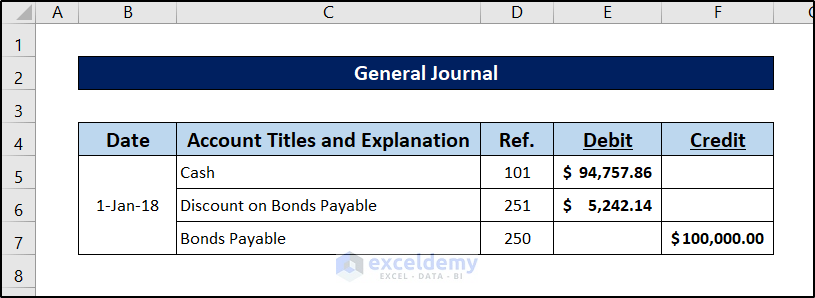
The company received a cash of amount $94,757.86. Debits increase assets: so, debit Cash $94,757.86.

It has to pay the $100,000 (face value of the bond) after 3 years (the maturity of the bond). So, $100,000 were credited to the account “Bonds Payable”.

In the “Discount on Bonds Payable” account, the discounted amount of the bond is adjusted.

It is a liability account and debits decrease a liability account, but they increase this Discount on Bonds Payable account. This is why it is called a contra account. The debit Discount on Bonds Payable is $5242.14.

Read More: How to Calculate Interest Rate from EMI in Excel

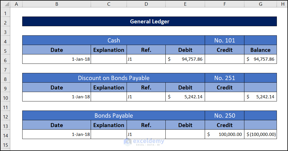
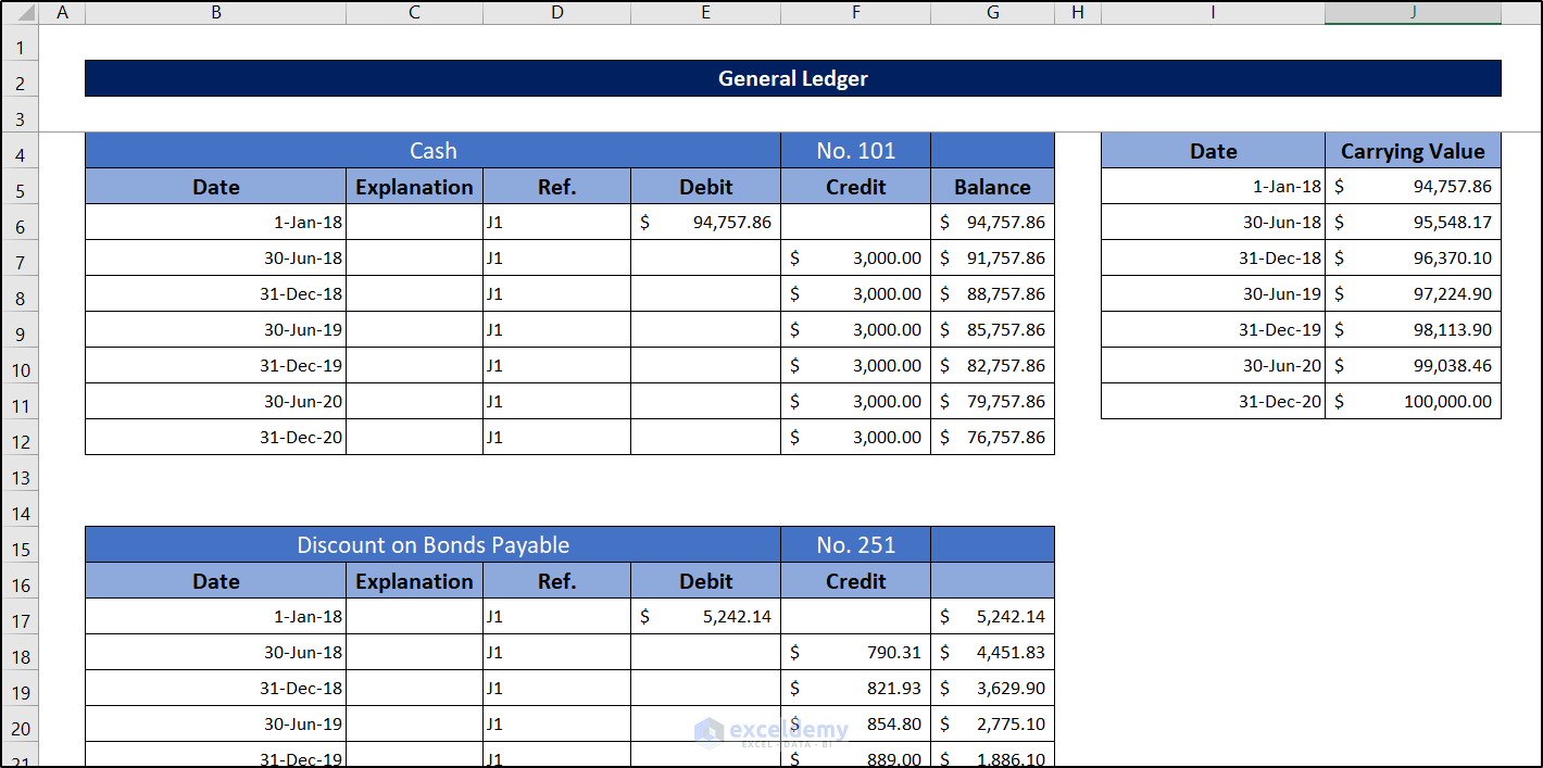
Step 2: Prepare a General Ledger

Rearrange the above data for the general ledger:

Step 3: Calculate the Carrying Value of the Bond

To calculate the carrying/book value of this bond, subtract the discounted amount from the bond face value.

On 1st Jan, 2018, the bond’s book value/carrying value = $100,000 – $5,242.14 = $94,757.86.

Over the next 3 years (the maturity of the bond), this book value will be adjusted: it will be $100,000 at the end of the maturity period.

This slow adjustment (also called amortization) of the book value to its face value can be done in two ways:

• Straight-line Method of Amortization
• Effective Interest Rate Method of Amortization

Consider the following transactions:

On 30th June 2018, the company is going to pay the bondholder his first semi-annual interest ($100,000 x 3% = $3000).

But the real Interest Expense = The book value of the bond x (market rate / 2) = $94757.86 x (8%/2) = $3790.31.

Debits increase the expense account. So, the Interest Expense account was debited $3790.31.

The company paid $3000 cash to the bondholder. Credits decrease the cash (asset) account. So, the credit cash is $3000.

The “Discounts on Bonds Payable” account is credited 790.31$. When liabilities decrease, they go into the debit column. But as this is a contra account, when liabilities decrease, they goes into the credit column.

The general ledger will be:

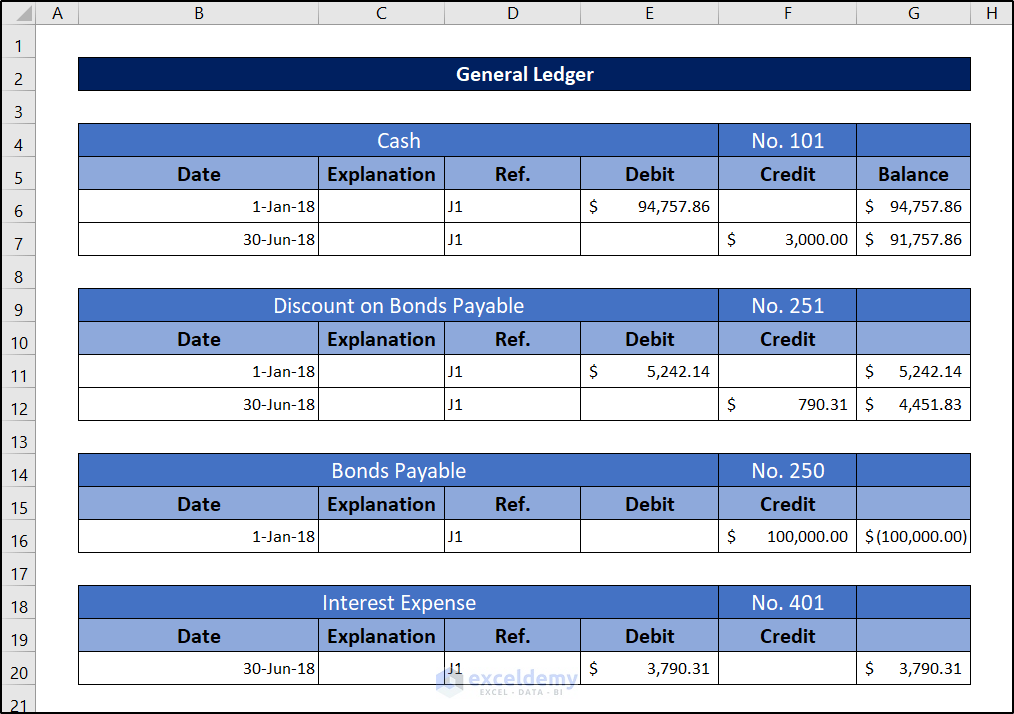
A new account (“Interest Expense”) was added to the “General Ledger”.

The company is paying (every 6 months): Face Value x (Nominal Interest Rate/2) = 100,000 x (6%/2) = $3000.

But there is a discount for the bond: its true return will be 8% every year (the market rate). So, there is a gap between the genuine cost of the fund and the given interest payments. In the “Interest Expense” account, the true cost of the fund was entered as $94757.86 x (8%/2) = $3790.31.

The difference between the true cost and the given interest payment (semi-annually) = $3790.31 – $3000 = $790.31.

This difference ($790.31) is credited to the Discount on Bonds Payable account.

Read More: How to Convert Monthly Interest Rate to Annual in Excel

Step 4: Record the Carrying Value

Consider a virtual account to keep the calculations of the carrying value (book value) of the bond.

The carrying value is the value on the basis of which the true cost of the fund is calculated.

On the issue date of the bond, its book value (carrying value) was $94757.86 (issue price)

After 6 months, the book value of the bond will be: $94757.86 + $790.31 = $95,548.17.

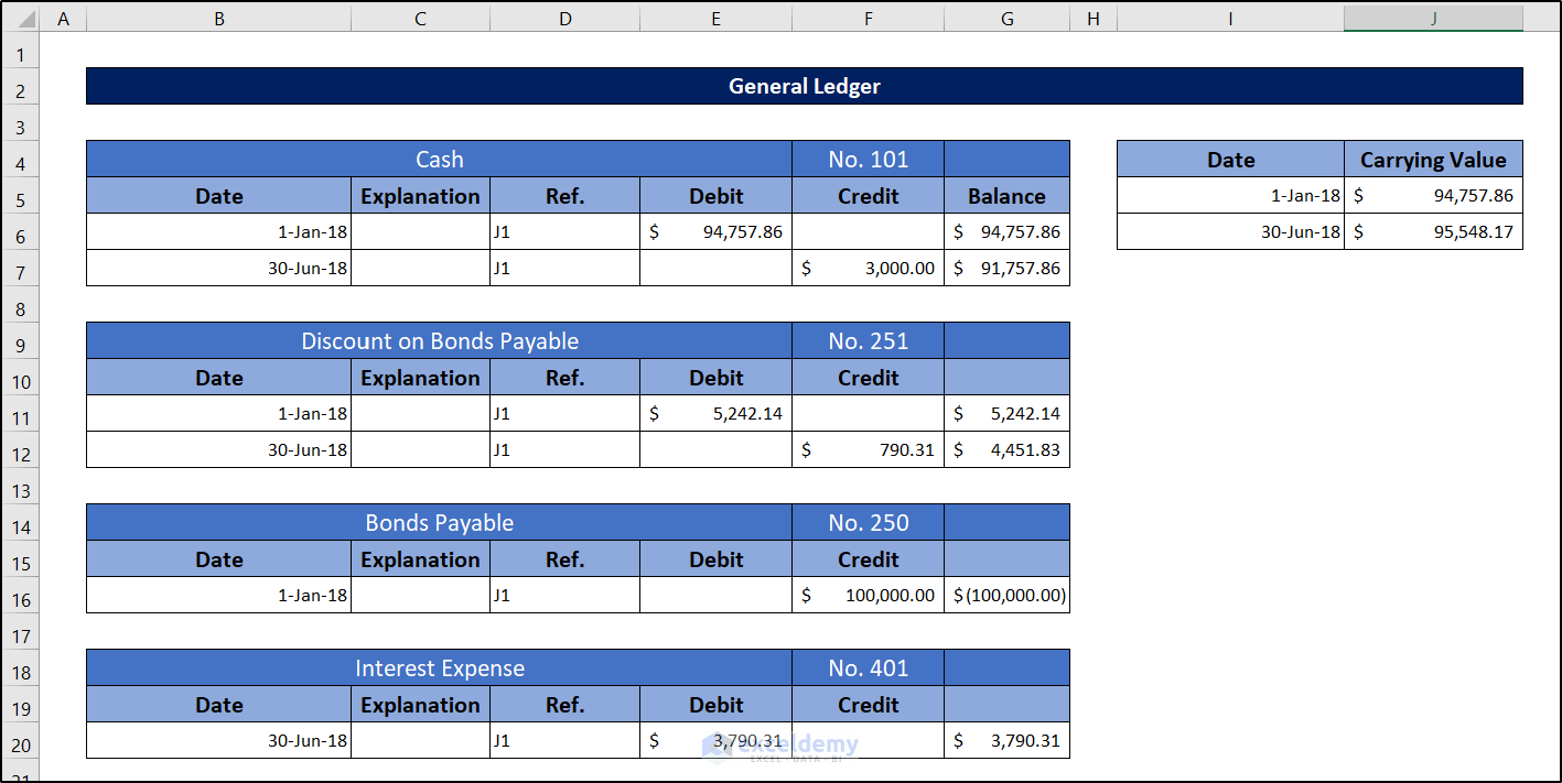
The true cost of the fund was $3790.31, but $3000 were paid to the bondholder. The remaining $790.31 was not in payment. So, the bondholder will get the interest for this unpaid amount at the market rate (8%).

After 6 months, the bond carrying value will be $95,548.17.

Step 5: Finalize the General Ledger

Repeat the steps for all the transactions. This is the final output.

This is the portion containing “Bonds Payable” and “Interest Expenses”.

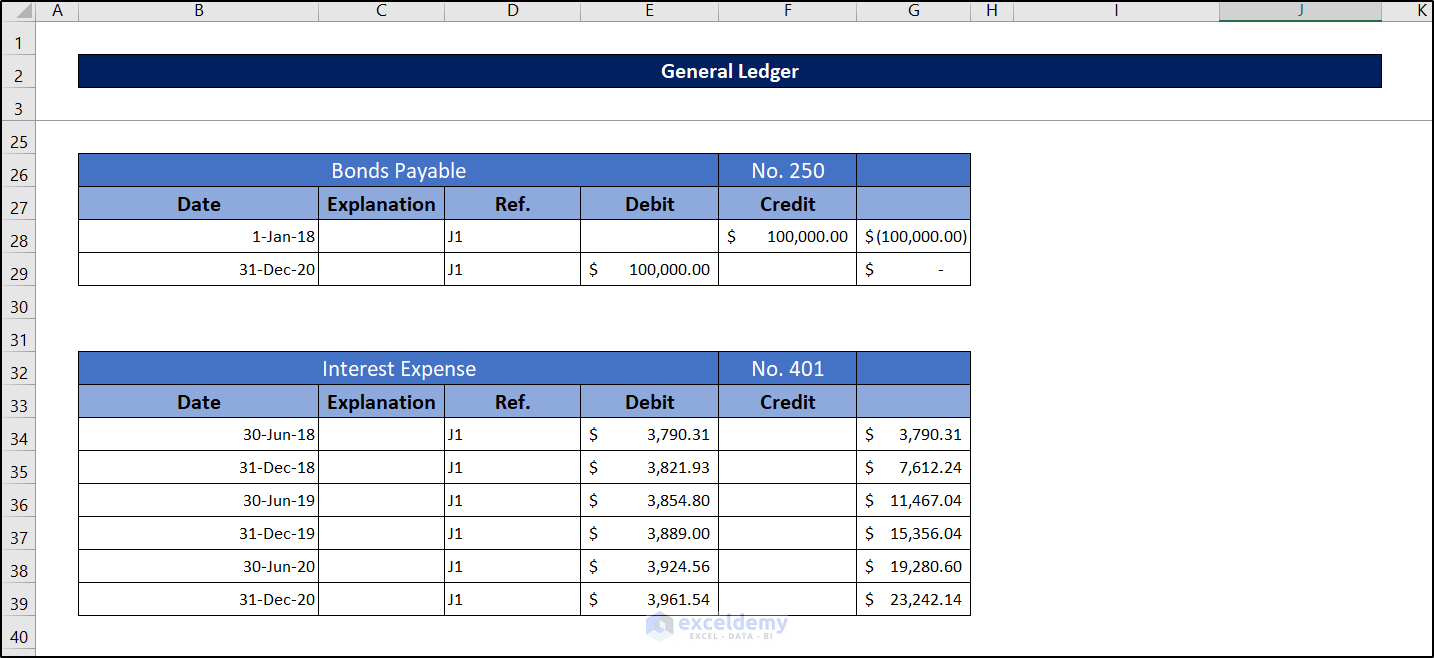
You can see that the total cash outflow from is: $76,757.86 – $100,000 = -$23,242.14. And this is the total “Interest Expense” for this bond in 3 years.

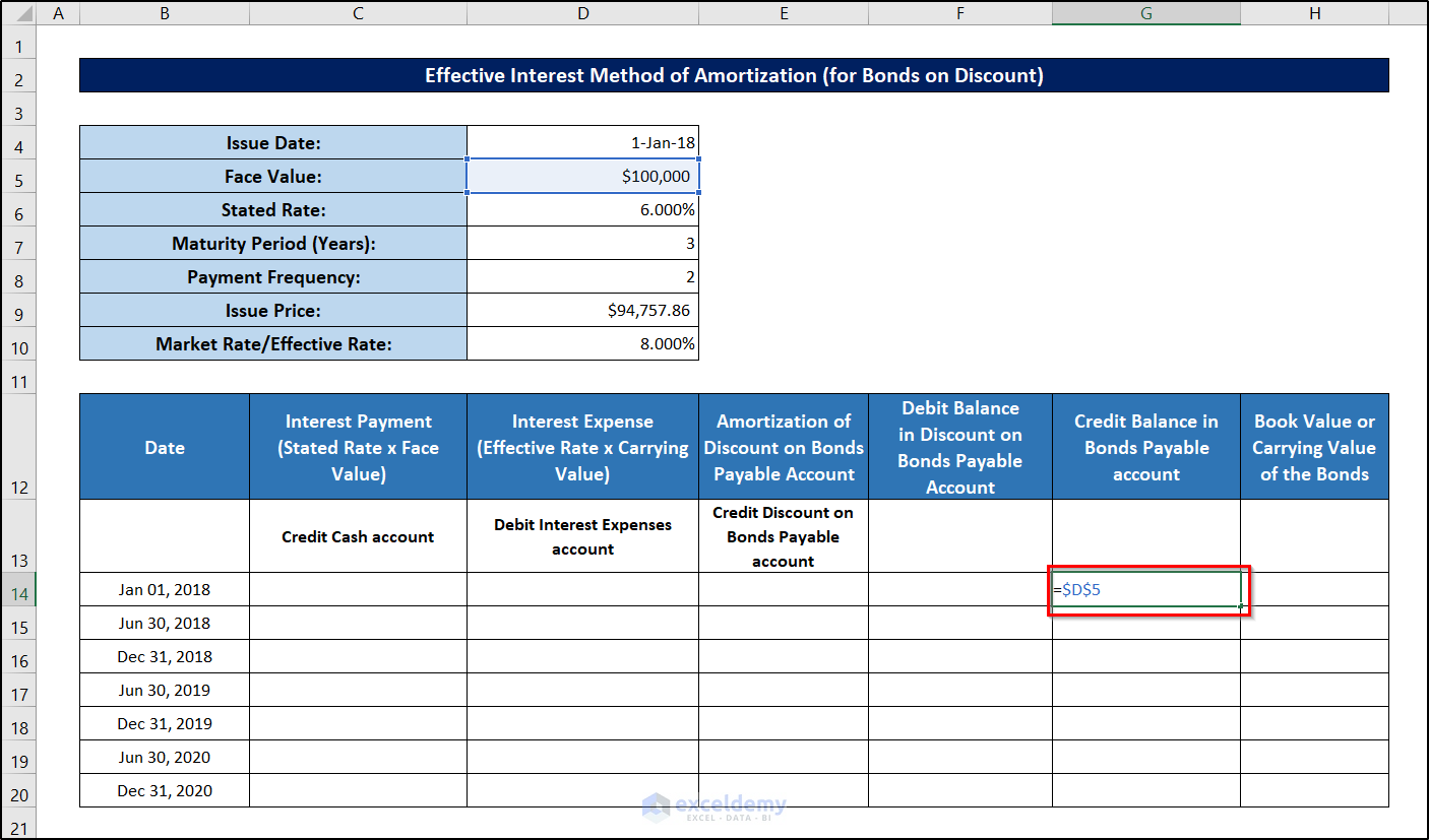
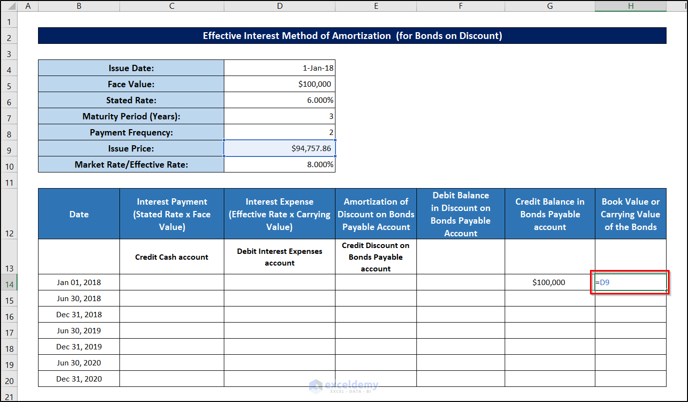
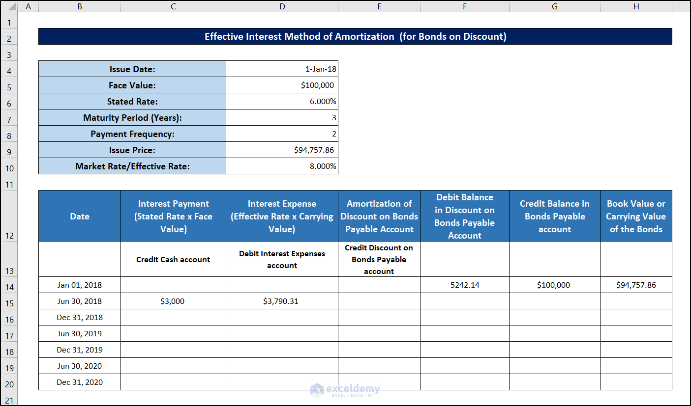
Step 6: Enter the Credit Balance and the Book Payable in the Amortization Table

Enter the data to create the amortization table format for the effective interest method.

Enter the credit balance using the following formula.

To enter the book value, use the following formula in H14.

Step 7: Calculate the Debit Balance

Use the following formula in F14.

Press Enter.

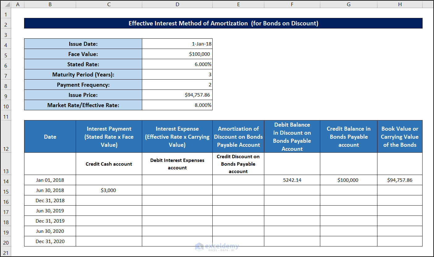
Step 8: Estimate the Interest Payment

Use the following formula in C15.

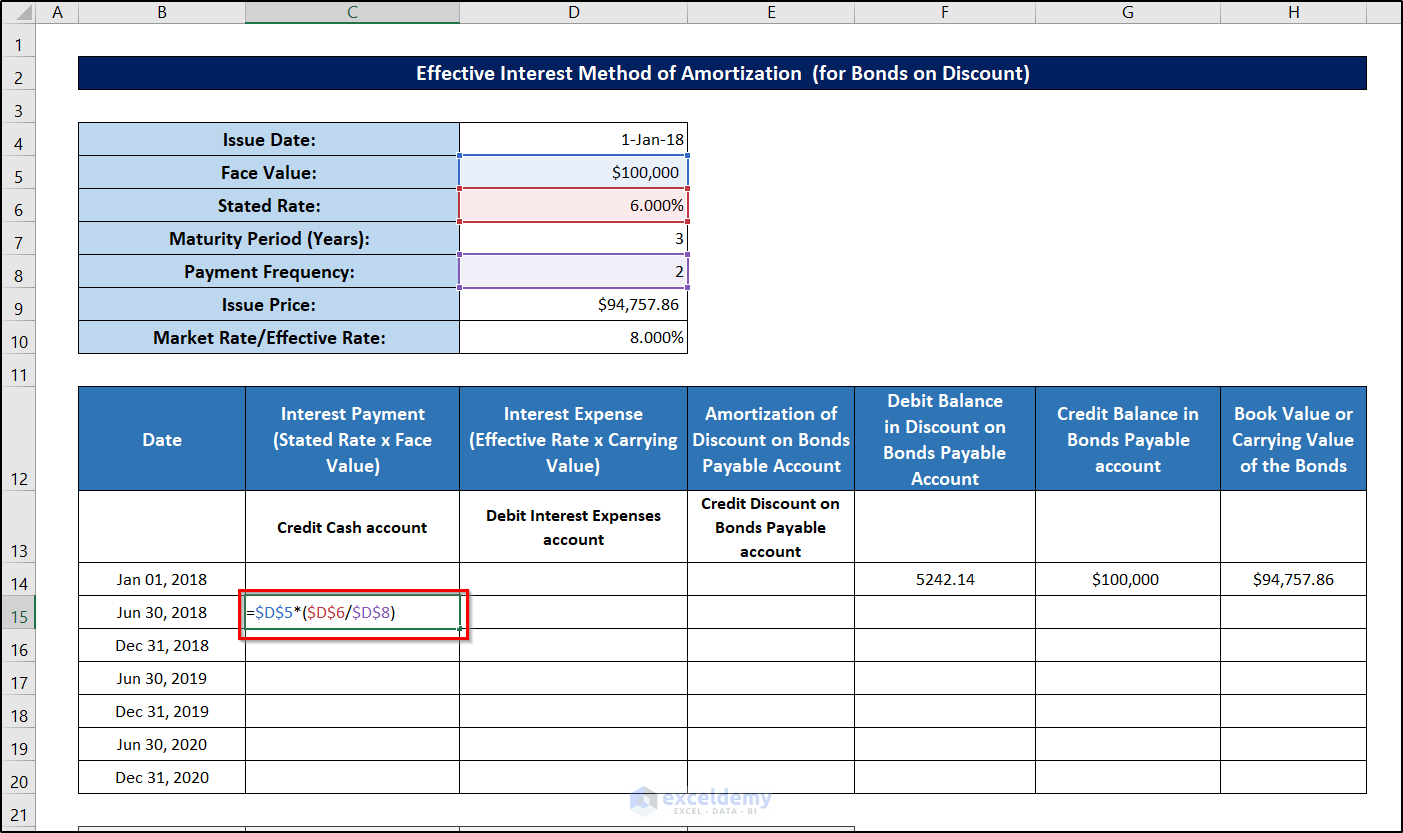
Press Enter.

Step 9: Compute the Interest Expense

Use the following formula in D15.

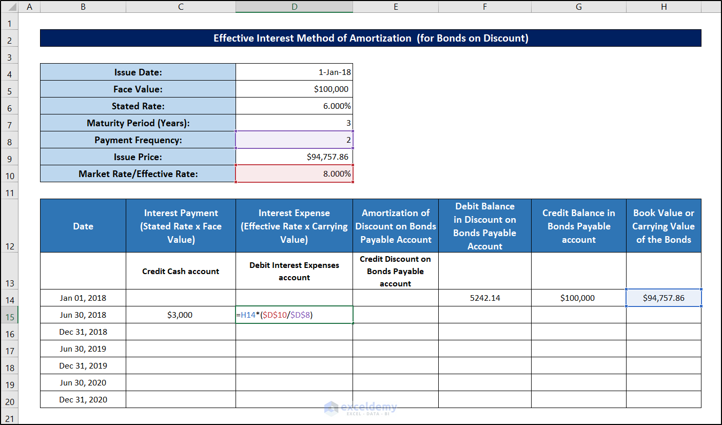
Press Enter.

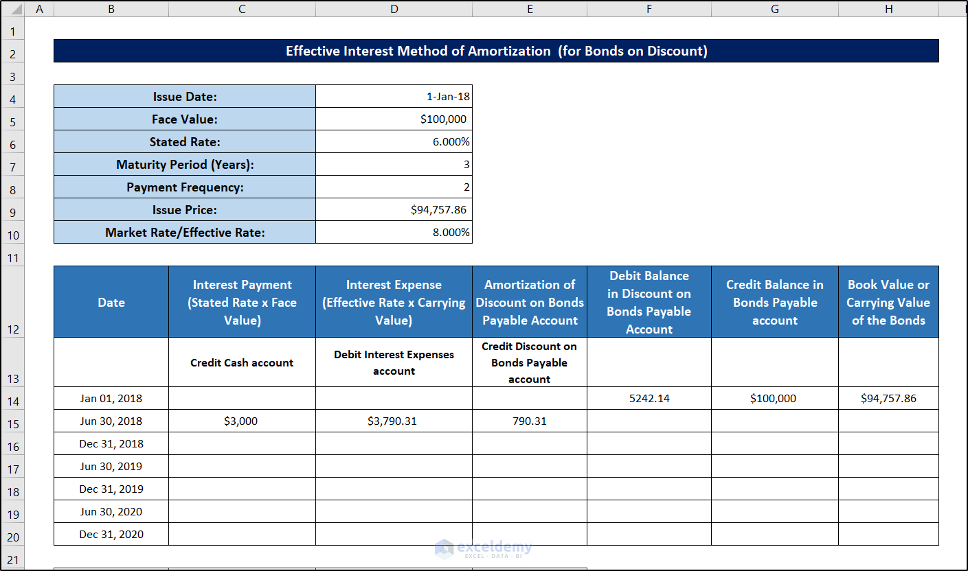
Step 10: Calculate the Amortization of Discounts on Bonds Payable

Chose column E and enter the following formula in E15.

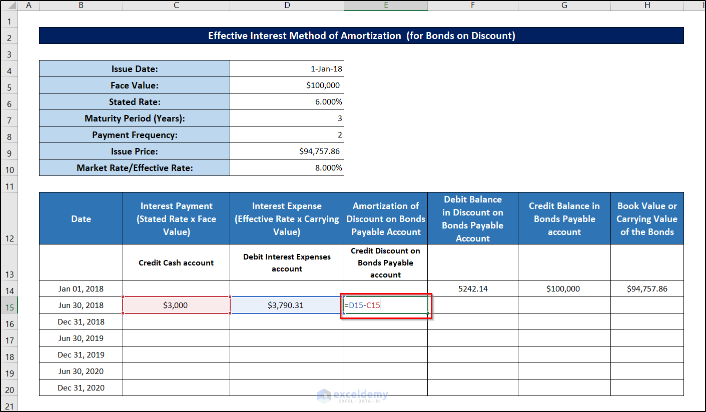
Press Enter.

Step 11: Enter the Rest of the Values

Click and drag the fill handle icon for all the cells in each column to fill the rest of the values.

Add formulas to calculate the total interest payments, interest expenses, and amortization. Use the SUM function.

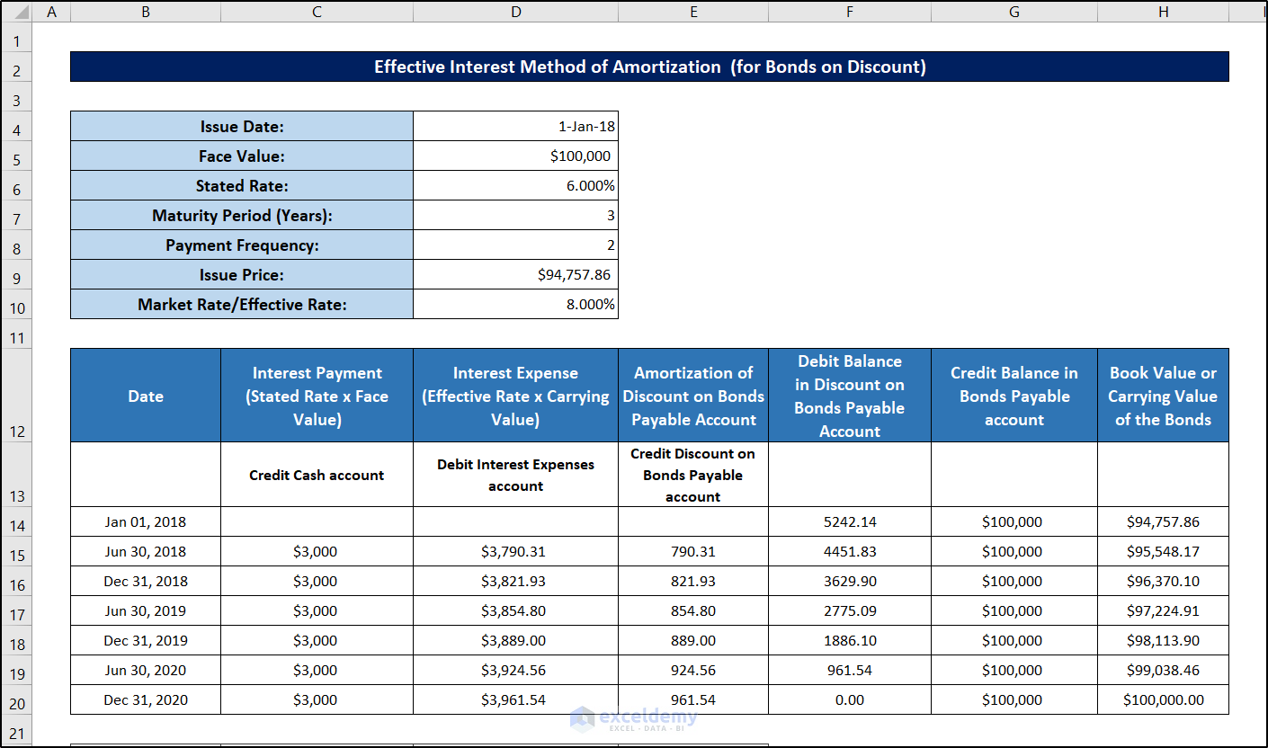
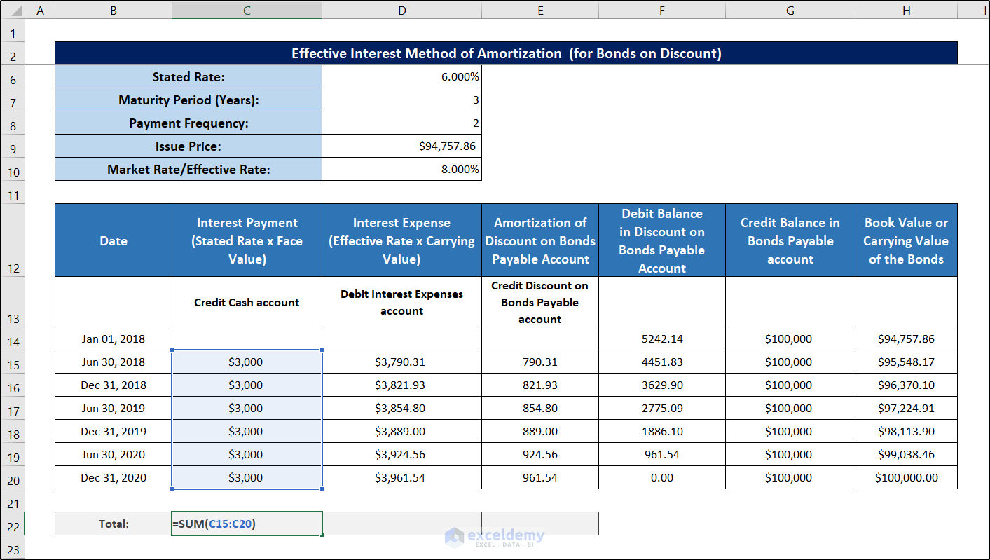
Enter the following formula in C22.

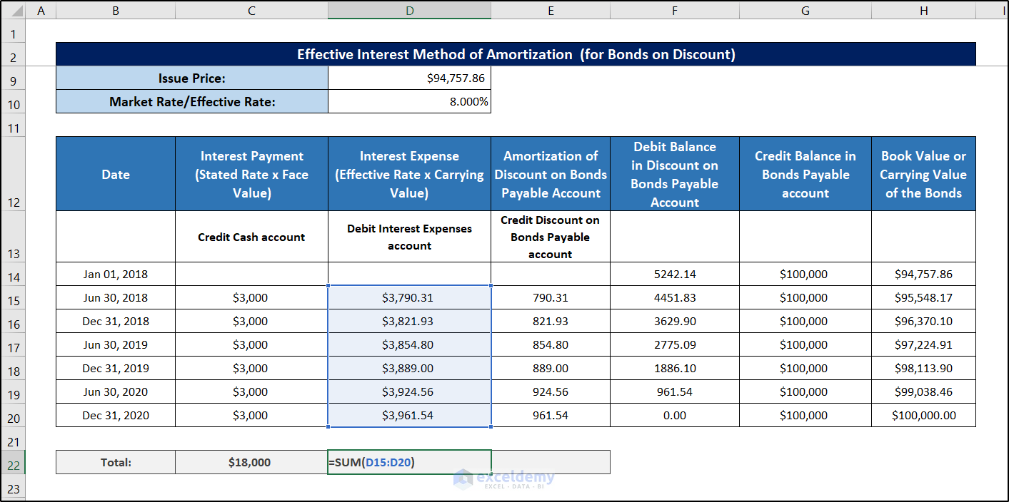
Use the following formula in D22.

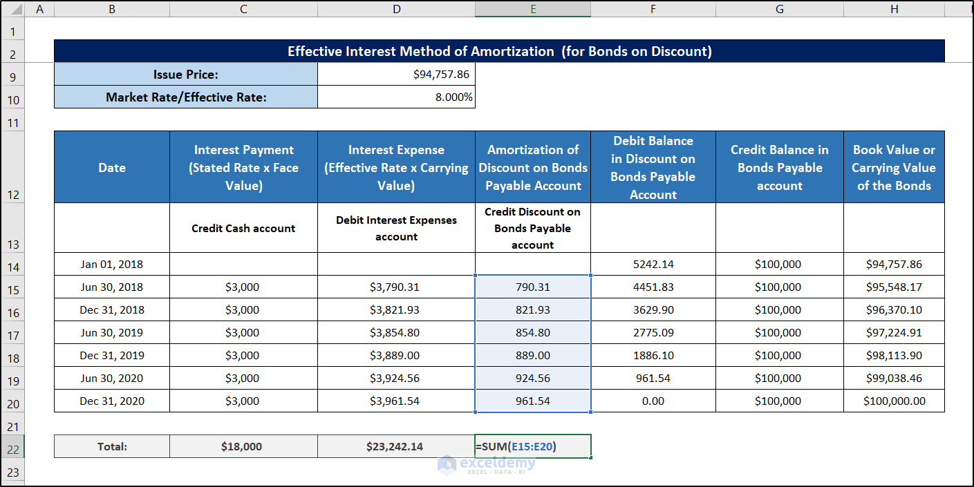
Enter the following formula in E22.

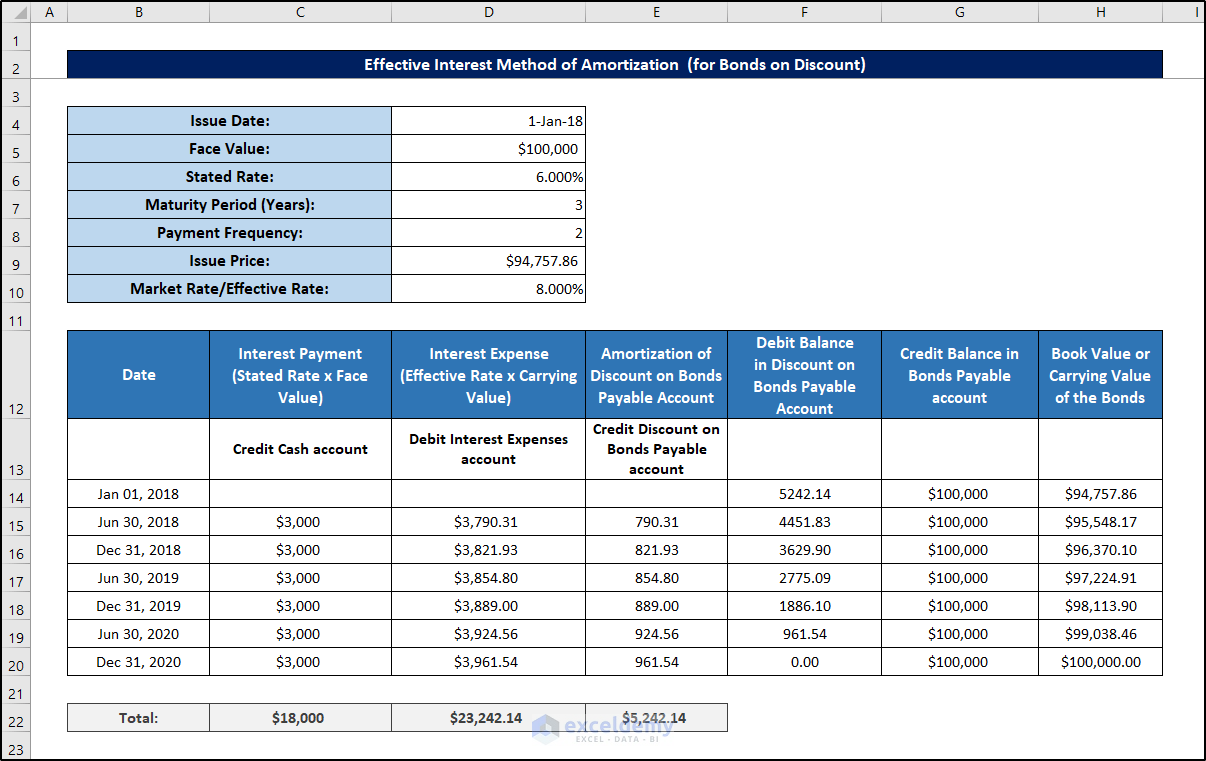
The amortization table for the effective interest method is complete.

Example 2 – Effective Interest Method of Amortization for Bonds Sold with Premiums

This is the amortization table for bonds sold with premiums.

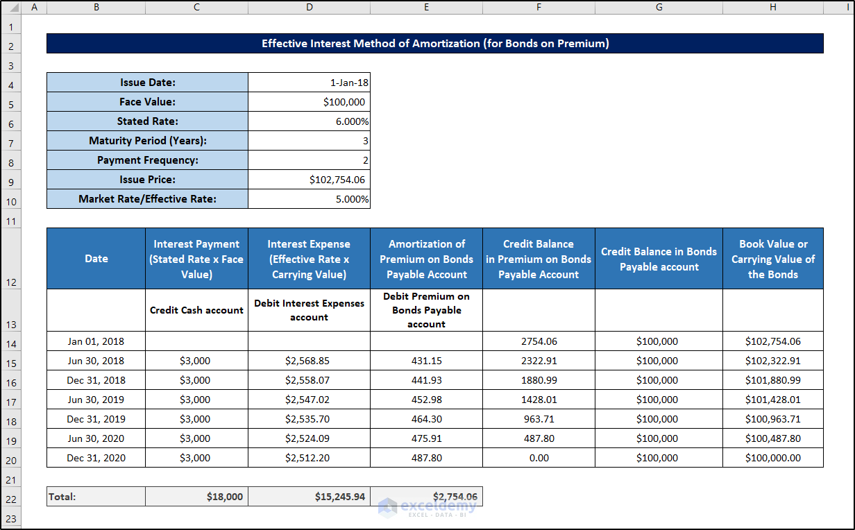
The steps are the same described in Example 1.

There’s a difference in calculations:

• For bonds that are sold in premium, you have to debit the Premium on Bonds Payable account gradually. It is not a contra liability account. You can call it an adjunct account because its purpose is to balance the additional amount received (for this bond: $102754.06 – $100000 = $2754.06).
• To calculate the carrying value of the bond subtract the additional interest (paid to the bondholder) from the current book value.

For example, on Jan 01, 2018, the carrying value of the bond was $102754.06. On June 30, 2018, $3000 were paid to the bondholder. But the cost of the fund ($102754.06) was $102754.06 x (5%/2 ) = $2568.85. The company is paying an extra amount: $3000 – $2568.85 = $431.15.

• Subtract this additional interest from the current carrying value of the bond to get the new carrying value: $102754.06 – $431.15 = $102322.91.

Read More: How to Calculate Monthly Interest Rate in Excel

Download Practice Workbook

Related Contents

• How to Calculate APR in Excel

<< Go Back to How to Calculate Interest Rate in Excel | Excel for Finance | Learn Excel