What Is Simple Interest?
Simple Interest doesn’t compound. In other words, Simple Interest is the interest calculated on the principal portion of a loan or the original contribution to a savings account. In addition, the account holder will gain interest only against the first deposit and the borrower will pay interest only on the initially borrowed amount.
Arithmetic Formula to Calculate Simple Interest
We will use a very straightforward formula to find Simple Interests.
I = p*r*t
I = Simple Interest
p= Principal Amount
r = Rate of Interest
t = Time elapsed
How to Calculate Simple Interest and Compound Interest in Excel: 2 Ways
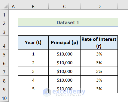
In the following dataset, we have a Principal Amount (p) that is deposited in the bank for 5 years. The bank will provide 3% Simple Interest each year. We will determine the interest amounts.
Method 1 – Using Arithmetic Formula
Steps:
- To calculate the Simple Interest for Year 1, use the following formula in cell E5.
=C5*B5*D5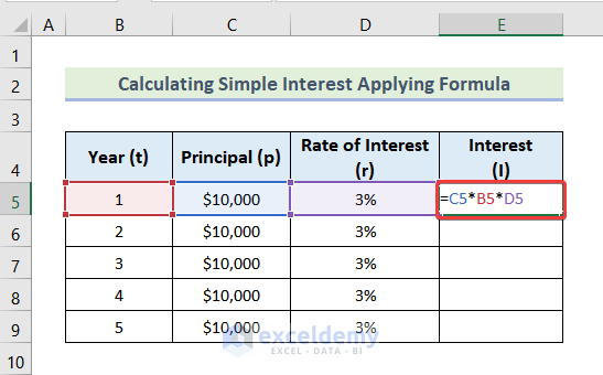
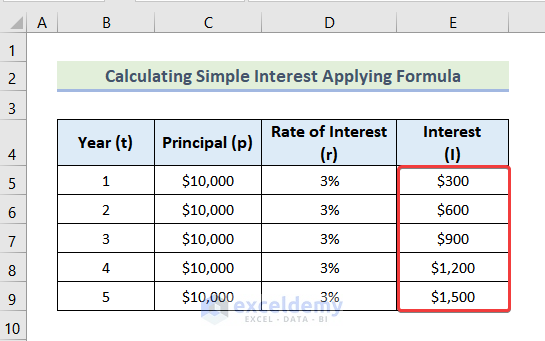
- Drag the Fill Handle to cell E9 and you will get the results for the remaining years.
Method 2 – Utilizing the FV Function to Calculate Simple Interest in Excel
Here, we are going to use the FV function (Future Value function). The function has the following arguments, in order:
- rate = rate of compounding interest
- nper = total number of payment periods
- pmt = amount of payment in each period
- pv = present value
- type = This indicates when payments are due. Use 0 for defining the end of the period and 1 for the beginning of the period.
In the case of Simple Interest, there is no Compounding Interest Rate. The rate in the FV function will be 0.
Steps:
- Use the following formula in cell E5.
=-FV(0,B5,(C5*D5),C5) 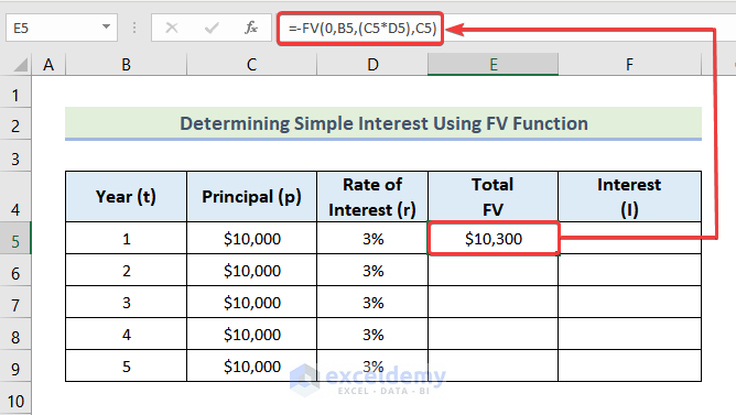
- Subtract the Principal (p) from the Total FV, and we will get the Interest (I). Use the formula in cell F5 to calculate our Simple Interest.
=E5-C5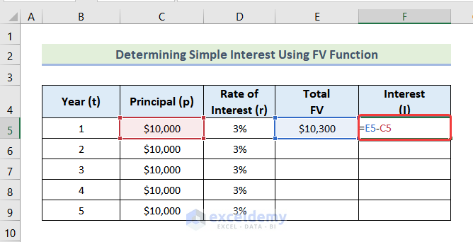
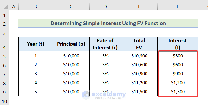
- Select cells E5 and cell F5 together.
- Drag the Fill Handle down.
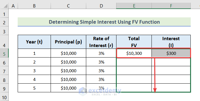
- Here are the results.
Read More: How to Calculate Simple Interest Loan Payments in Excel
What Is Compound Interest?
Compound Interest is when you earn interest on your interest. When you put money into a savings account that earns Compound Interest, you will get interest on both the money you put in and the interest that builds up over time.
Arithmetic Formula to Calculate Compound Interest
We will use the following formula to calculate Compound Interest.
CI = p(1+r/n)^nt
CI = Compound Interest
p = Principal Amount
r = Rate of Compound Interest
n = Number of compoundings per unit time
t = Time
2 Methods to Calculate Compound Interest in Excel
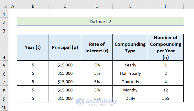
We have a Principal Amount (p) deposited in a bank with a 5% Compounding Interest Rate. In the data set, we have 5 types of compoundings. They are:
| Compounding Type | Number of Compounding Per Year (n) | Explanation |
|---|---|---|
| Yearly | 1 | Once a year |
| Half – Yearly | 2 | Once every 6 months ( 2 times a year) |
| Quarterly | 4 | Once every 3 months ( 4 times a year) |
| Monthly | 12 | Once every month ( 12 times a year |
| Daily | 365 | Once every day ( 365 times a year) |
We’ll calculate the Compound Interests for these different types of compounding.
Method 1 – Using Arithmetic Formula
Steps:
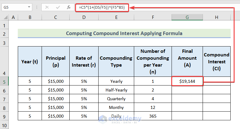
- Use the following formula in cell G5.
=C5*(1+(D5/F5))^(F5*B5)Cell F5 denotes the cell of Number pf Compounding Per Year, and cell G5 represents the cell of Final Amount.
- To get the Compound Interest (CI) we need to subtract the Principal from the Final Amount. Use the following formula in cell H5.
=G5-C5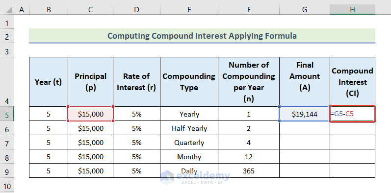
- Select cells G5 and cell H5 together.
- Drag the Fill Handle down or double-click it.
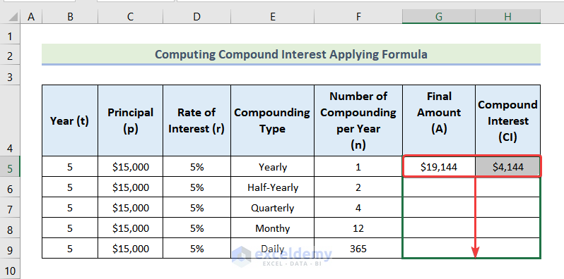
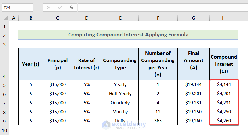
- Here’s the result.
Method 2 – Applying the FV Function to Calculate Compound Interest in Excel
Steps:
- Use the following formula in cell G5.
=FV(D5/F5,B5*F5,0,-C5)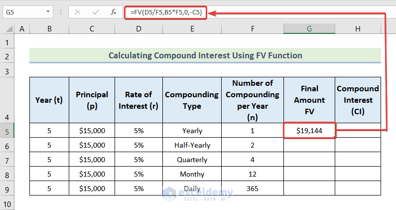
- Use this formula in cell H5.
=G5-C5
- Choose cells G5 and cell H5.
- Double-click the Fill Handle or drag it down.
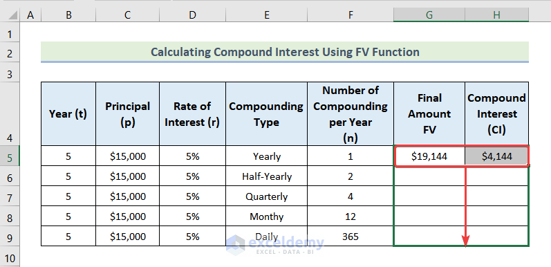
- You’ll get all the results.
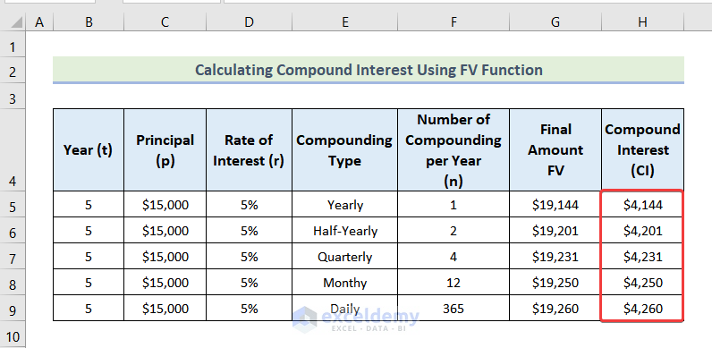
Things to Remember
- While using the FV function to Calculate Simple Interest, make sure you put a negative sign before it. Excel considers it as cash outflow.
- Put a negative sign before the Present Value while computing Compounding Interest Using the FV function.
Download the Practice Workbook
Related Articles
- Convert Compound Interest to Simple Interest in Excel
- How to Calculate Simple Interest on Reducing Balance in Excel
<< Go Back to Simple Interest Formula in Excel | Excel for Finance | Learn Excel
Get FREE Advanced Excel Exercises with Solutions!
