Step 1 – Prepare the Dataset
- Insert the product names in the Product column.
- Insert the manufacturing date in the MFG Date column.
- Provide the information on the length of use in the Duration of Usage column.
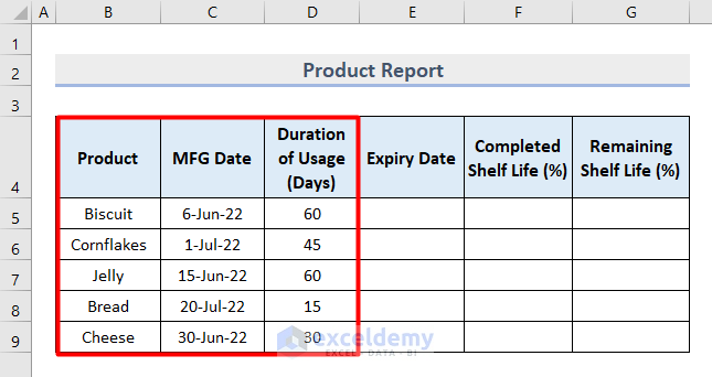
- Make sure you define the unit of duration. We put all durations in Days.
Read More: Make an Excel Spreadsheet Automatically Calculate Percentage
Step 2 – Calculate the Date of Expiration in Excel
- Insert this formula in cell E5:
=C5+D5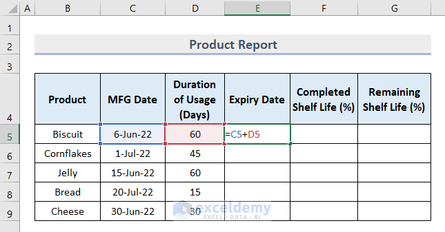
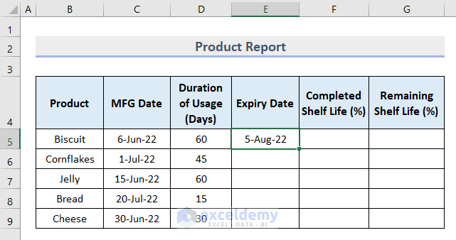
- Press Enter.
- You will see the expiry date of the first product based on the MFG Date and duration.
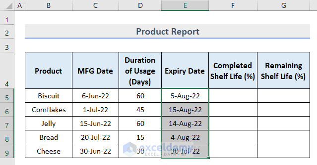
- Use the Fill Handle tool to drag this formula in the cell range E6:E9.
Additional Tip: If your duration of usage is in weeks, months or years, apply these formulas for each type of duration.
- For 3 weeks:
=E5+3*7 - For 3 months:
=EDATE(E5,3) - For 3 years:
=DATE(YEAR(E5)+3,MONTH(E5),DAY(E5))
Step 3 – Find Out the Percentage of Completed Shelf Life
- Insert this formula in cell F5:
=YEARFRAC(C5,E5,1)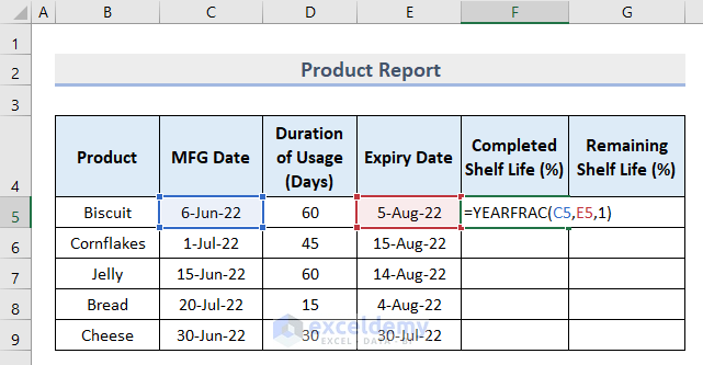
- Press Enter.
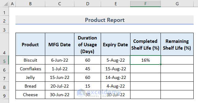
We used the YEARFRAC function to calculate the value of duration between the manufacturing date and the expiry date in fractions.
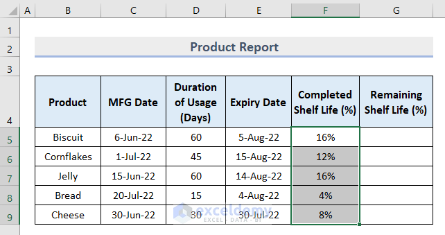
- Format the cell as a percentage.
- Apply this formula in the cell range F6:F9 using the AutoFill tool.
Step 4 – Calculate the Remaining Shelf Life Percentage
- Insert this formula in cell G5.
=1-F5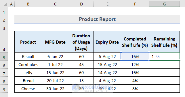
- Hit Enter.
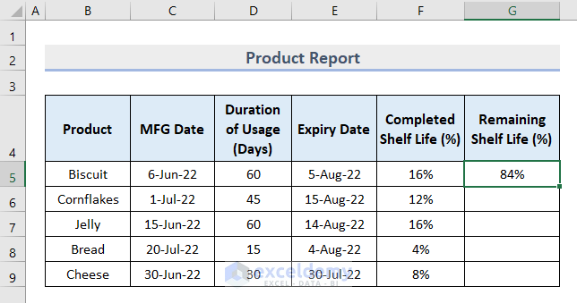
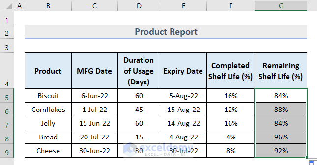
- Drag the bottom corner of cell G5 down to cell G9 to get the value for each product.
Step 5 – Check the Expiration Status in Excel
- Insert today’s date in cell D11. We inserted the present day as 10 August 2022 for calculation.
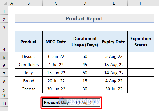
Note: You can use the TODAY function to find the present day based on your region. Simply apply this formula in cell D11.
=TODAY()- Insert this formula in cell F5.
=IF($D$11>E5,"Expired",(E5-$D$11))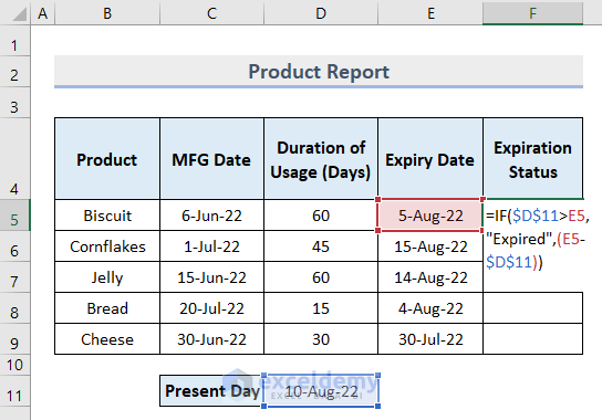
- Press Enter.
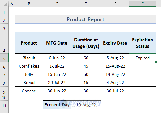
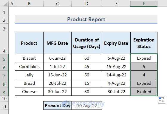
We used the IF function to make a comparison between the values of cells D11 and E5. The output will be Expired if the former is earlier.
- Apply this formula in cell range F6:F9 and you will get the final output.
Things to Remember
- Make sure you insert the dates in the Date format before calculation.
- Format the result cell in the Percentage format.
- If you want to find the Duration of Usage, apply this formula:
=Expiry Date - MFG Date- Mind the blank cells in your dataset. Otherwise, it will show a false result.
Download the Practice Workbook
Related Articles
- How to Calculate Error Percentage in Excel
- How to Calculate Cumulative Percentage in Excel
- How to Calculate Mean Percentage Error in Excel
- How to Calculate Percentage of Completion in Excel
- How to Calculate Percentage of Budget Spent in Excel
- How to Calculate Utilization Percentage in Excel
- How to Calculate Absenteeism Percentage in Excel
- How to Calculate Savings Percentage in Excel
- How to Calculate Productivity Percentage in Excel
- How to Calculate Variance Percentage in Excel
- How to Calculate Accuracy Percentage in Excel
- How to Calculate Grade Percentage in Excel
- How to Calculate Win-Loss Percentage in Excel
- How to Calculate SLA Percentage in Excel
<< Go Back to Percentage Formula Examples | Calculating Percentages | Calculate in Excel | Learn Excel
Get FREE Advanced Excel Exercises with Solutions!
