Sometimes, you may need to calculate percentage range, percentage relative range, or percentage of cells in a range. Microsoft Excel enables you to perform this type of task in bulk. This article demonstrates how to calculate percentage range in Excel and also percentage relative range and percentage of cells in a range.
What Is Percentage Range?
Percentage range generally means a range of percentage which is normally represented between two percentage values. For example, 80%-100% marks in an exam represent grade A. So, 80%-100% is the percentage range here.
Calculate Percentage Range in Excel Using IF Function
Suppose, you have a datasheet where you have the marks of students. In this case, the total marks are 120 and you want to find out their percentage range (100%, 80%-99%, 33%-79%,0%-32%). Now, I will show you how to do so using the IF function.

Here, follow the steps below to calculate the percentage range.
Steps:
- First, add a column for the percentage range.
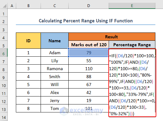
- Now, select the D6 cell and type the following formula.
Here, D6 is the first cell of the Marks out of 120 columns.
⧬ Formula Explanation
In this formula, the IF function is used.
- Here, the first logical test is to check if (D6/120)*100 is equal to 100. If true, it gives an output of 100% and if false, it moves to the second logical test.
- Now, the second logical test checks if (D6/120)*100>=80,(D6/120)*100<100. If true, it gives an output of 80%-99% and if false, it moves to the third logical test.
- In the third logical test, it checks if (D6/120)*100>=33,(D6/120)*100<80. If true, it gives an output of 33%-80% and if false it moves to the fourth and final logical test.
- At last, the formula checks if (D6/120)*100>=0,(D6/120)*100<33). If true, it returns an output 0% to 32%.
- Now, press ENTER and it will show you the output.
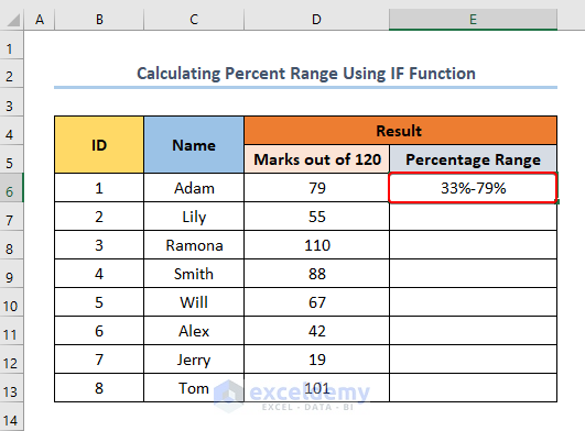
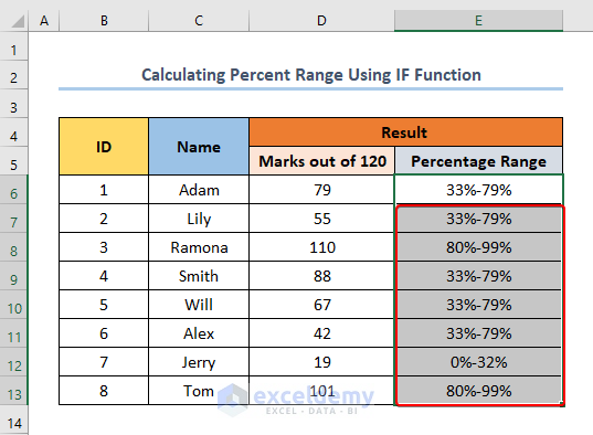
- Finally, drag the Fill handle for the rest of the column.
What Is the Percentage Relative Range?
Percentage Relative Range is defined by the ratio of the range of percentages to the average of them. Stock market enthusiasts generally calculate this parameter to get an idea about a stock.
Arithmetic Formula to Calculate Percentage Relative Range
The arithmetic formula to calculate the percentage relative range is as follows:
P=((H-L)/((H+L)/2))*100
Here,
P = Percentage Relative Range (%)
H= Higher Value
L= Lower Value
How to Calculate Percentage Relative Range in Excel
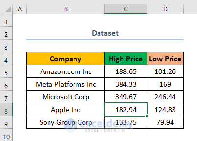
Suppose, you have a list of companies and their highest stock price and lowest stock price for a fifty two weeks period . Now, you want to calculate their percentage relative range. I will show you two methods to do so.
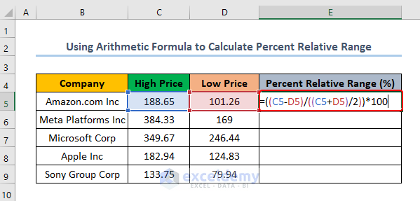
1. Using Arithmetic Formula to Calculate Percentage Relative Range
Using the arithmetic formula and inserting it manually is one of the fastest and most convenient ways to calculate the percentage relative range. At this point, follow the steps below to calculate the percentage relative range.
Steps:
- First, add a column for Percent Relative Change.
- Next, select cell E5 and put in the following formula.
Here, E5 is the first cell of the column Percent Relative Range (%). Also, C5 and D5 are the first cells for High Price and Low Price respectively.
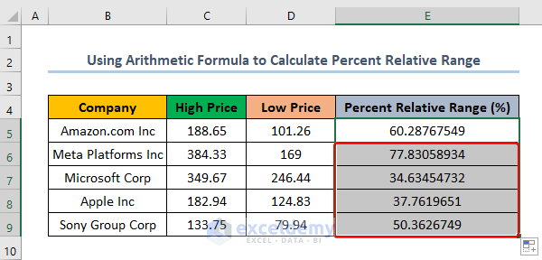
- After that, press ENTER and you will get your output.

- Lastly, drag the Fill handle for the rest of the column.
Read More: How to Calculate Range for Grouped Data in Excel
2. Applying VBA Code to Calculate Percentage Relative Range
You can also use VBA code to create a function for VBA and then use it to calculate Percentage Relative range. Now, I will show you how to do so in two sets of steps. In the first set of steps, you will create a function using VBA. Then, in the following set of steps, you will calculate the percentage relative range by using the function.
Steps 01:
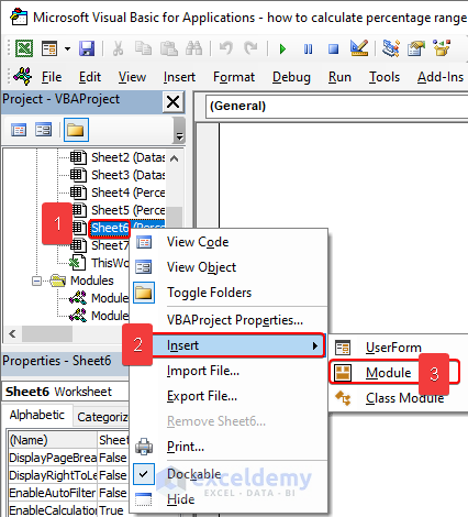
- First, press ALT + F11 to open the VBA
- Now, select Sheet 6 and Right-Click on it.
- Next, sequentially select Insert > Module.
- After that, copy the following code and paste it into the blank space.
'Function for calculating Percent Relative Range
Public Function PercentRelativeRng(high, low)
Avg = (high + low) / 2
Rng = high - low
PercentRelativeRng = (Rng / Avg) * 100
End Function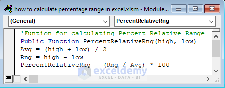
- Now, press F5 to run the code. Eventually, this code will create a function “PercentRelativeRng” which will help you to calculate the percentage relative range. This function has High Price as the first argument and Low Price as the second argument.
Steps 02:
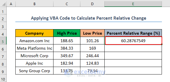
- After creating the new function, select the cell E5 and insert the following formula:
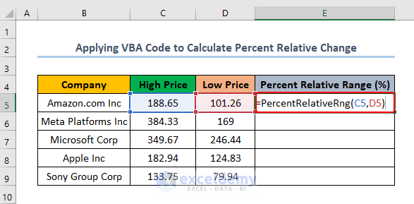
- At this point, press Enter and you will get your output.
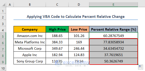
- Finally, drag the Fill handle for the remaining column.
Read More: How to Calculate Moving Range in Excel
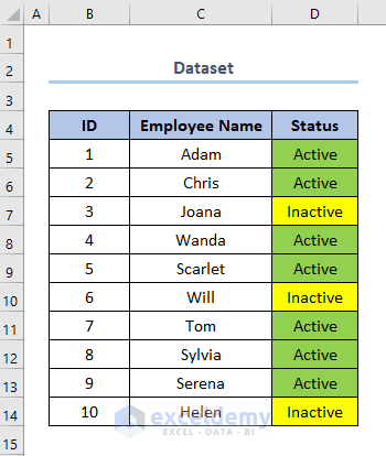
How to Calculate Percentage of Cell Range
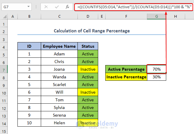
Suppose you have a dataset of active and inactive employees. Now, you want to know what percentage of them were active and which were inactive. You can do this easily by using Excel. Now, follow the following steps to do so.
Steps:
- First, select cell G7 and put in the following formula.
Here, G7 is the cell denoting the Active Percentage. D5 and D14 are the first and last cells of the Status column.
⧬ Formula Explanation :
In this formula,
- The (COUNTIFS(D5:D14,”Active”) syntax counts the number of people active.
- The syntax (COUNTA(D5:D14))) counts the number of inactive people.
- Multiplying it by 100 converts it into percentage.
- Lastly, ‘& “%”’ adds a % sign at the end.
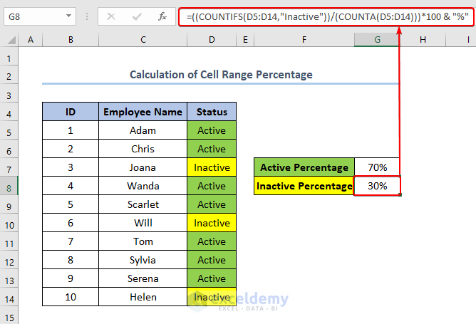
- Similarly, select cell G8 and put the following formula.
Here, G8 indicates the Inactive Percentage.
Download Practice Workbook
You can download the practice workbook from the link below.
Conclusion
Last but not the least, I hope you found what you were looking for from this article. If you have any queries, please drop a comment below.
Related Articles
- How to Calculate Time Range in Excel
- Calculate Interquartile Range in Excel
- How to Calculate Bin Range in Excel
<< Go Back to Range Formula in Excel | Excel Range | Learn Excel
Get FREE Advanced Excel Exercises with Solutions!
