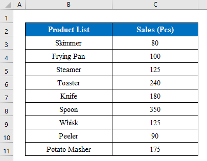
We have a dataset of some Product List and their Total Sales in quantity. We are going to calculate the moving range using formulas.
Method 1 – Apply the AVERAGE Function to Calculate the Moving Range in Excel
Steps:
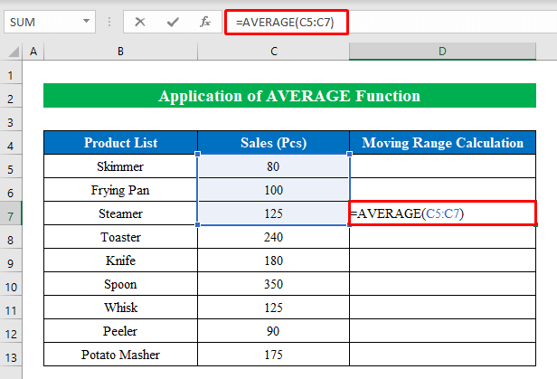
- Choose a cell to apply the formula. Here, I have selected cell (D7) as we take 3 intervals to get out the moving range value.
- Enter the following formula:
=AVERAGE(C5:C7)Where,
- The AVERAGE function returns the average value inside a given string. Here, we have provided the cells (C5:C7); thus, the average value for the cells is “67.”
- Press Enter to get the output.
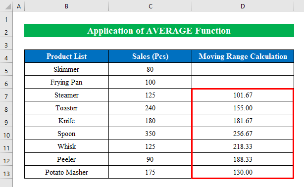
- Drag down the “fill handle” to fill all the cells with the moving range.
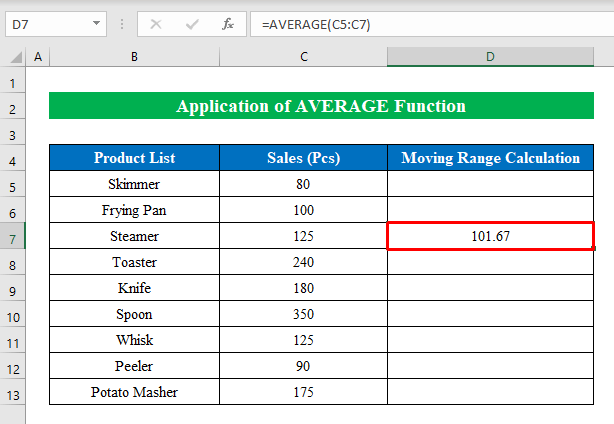
We have successfully calculated the moving range, indicating the average sales quantity from the product list.
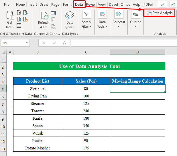
Method 2 – Use the Data Analysis Tool to Calculate Moving RangeSteps:
- Press the “Data Analysis” option from the “Data” option.
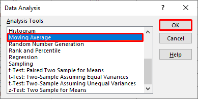
- A new dialog box named “Data Analysis” will appear.
- From the new window, choose “Moving Average” and press OK to continue.
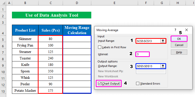
- In the new dialog box, choose your “Input Range” cells (C5:C13).
- Choose an interval as we determine the average value with 3 values. We put “3” in the “Interval” section.
- Select the “Output Range” from your dataset to view your calculated output.
- Check mark the “Chart Output” if you want to get the chart in your worksheet.
- Press OK.
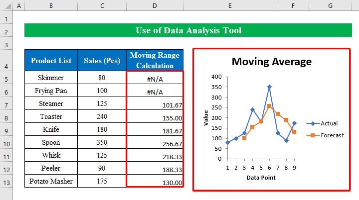
- We have the moving range values in our selected output cells with a chart.
Method 3 – Calculate the Moving Range for the Last N-th Values in Excel
Steps:
- Choose a cell (D13) to apply the formula.
- Enter the following formula:
=AVERAGE(OFFSET(C5,COUNT(C5:C100)-3,0,3,1))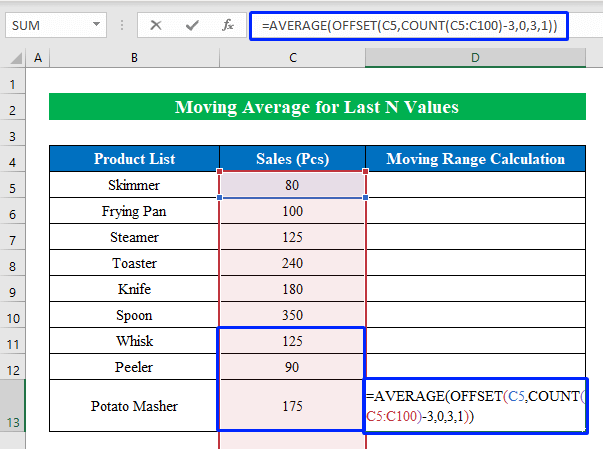
Formula Breakdown:
- COUNT(C5:C100)→ In this part the COUNT function is counting how many values are available in Column C and providing an output-”9” as we have a total of 9 values in the column.
- OFFSET(C5,COUNT(C5:C100)-3,0,3,1)→ The OFFSET function takes the cell reference C5 and then selects the range by taking the starting and ending point from the argument to calculate.
- Here, “-3” indicates 3 rows up, “0” order to stay in the same column, “3” means consisting of total 3 rows, and “1” indicates a total of 1 column.
- AVERAGE(OFFSET(C5,COUNT(C5:C100)-3,0,3,1))→ In the end, the AVERAGE function returns the average value from the selected cells in the range.
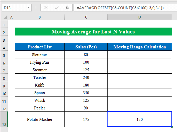
- Press the Enter button.
- We have successfully calculated the moving range for the last 3 cells in Excel.
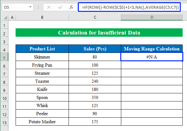
Method 4 – Calculate the Moving Range for Insufficient Data in Excel
Steps:
- Choose a cell (D5) and enter the following formula:
=IF(ROW()-ROW($C$5)+1<3,NA(),AVERAGE(C5:C7))Where,
- The IF function generates values with the help of the ROW and AVERAGE functions. If the value for this argument “ROW()-ROW($C$5)+1” is less than “3,” then show “#N/A,” and if not, display the average value.
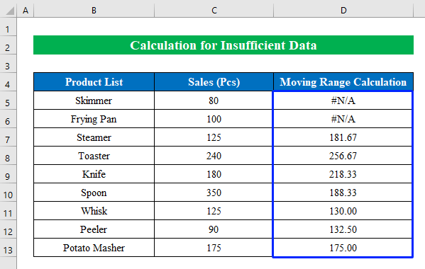
- Press Enter and drag the “fill handle” down to fill all the cells.
- We have the moving range output in our hands using a simple formula.
Things to Remember
- If you haven’t enabled the “Data Analysis” option, you won’t be able to enjoy the fantastic feature. To enable it, go to File > Options > Add-ins. From there, choose “Analysis Toolpak” and click OK. That’s it.
Download the Practice Workbook
Download this workbook to practice.
Related Articles
- How to Calculate Interquartile Range in Excel
- How to Calculate Percentage Range in Excel
- How to Calculate Time Range in Excel
- How to Calculate Bin Range in Excel
<< Go Back to Range Formula in Excel | Excel Range | Learn Excel
Get FREE Advanced Excel Exercises with Solutions!
