There are several methods to calculate the correlation coefficient in Excel. Among them, we will demonstrate to you 3 simple, easy, and effective methods
Basics of Correlation Coefficient
The correlation coefficient defines the strength of the relationship between two variables.
There are 3 types of correlation between data, these are positive correlation, negative correlation, and no relationship.
Positive correlation coefficient defines that when one variable increases, another variable also increases. The value of the positive correlation coefficient is greater than 0.
Negative correlation coefficient defines that when one variable increases, another variable decreases. The value of the negative correlation coefficient is less than 0.
No relationship correlation coefficient defines that there is no relationship between two variables, and the value is close or equal to 0.
How to Calculate Correlation Coefficient in Excel: 3 Methods
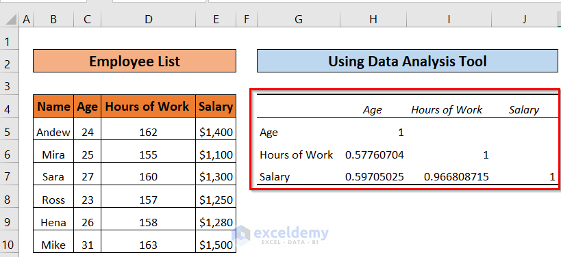
The following Employee List table shows the Name, Age, Hours of Work, and Salary columns. We will find out the correlation coefficient between Age, Hours of Work, and Salary. Here, we used Excel 365. You can use any available Excel version.

Method-1: Using CORREL Function to Calculate Correlation Coefficient
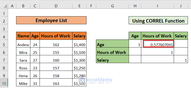
Here, in the following using CORREL Function table, we will calculate the correlation coefficient by using the CORREL function. In cells H5, I6, and J7 we put the value 1, as the correlation coefficient between two same variables is 1. Now, we have to calculate the correlation coefficient for the other cells.

➤ First of all, to find the correlation coefficient between Age and Hours of Work, we have to type the following formula in cell I5.
=CORREL(C5:C10,D5:D10)Here, the CORREL function returns the correlation coefficient of two cell ranges.
C5:C10 is array 1, and D5:D10 is array 2.
➤ After that, press ENTER.

Now, we can see the correlation coefficient in cell I5, the value is greater than 0. Hence, we know that the correlation coefficient between Age and Hours of Work is positive.
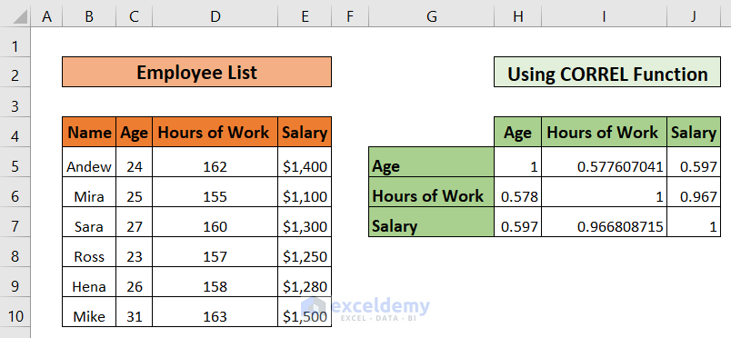
➤ In a similar way, we use the CORREL function in other cells to find out the correlation coefficient between variables.
Finally, we can see the result in the following using the CORREL Function table.
Method-2: Calculate Correlation Coefficient Using Data Analysis Tool
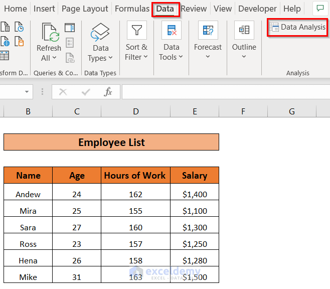
We can calculate the correlation coefficient in a quicker and easier way by using the Data Analysis tool. In this method, we’re going to use that analysis tool to calculate the coefficient.
➤ First of all, we will go to the Data tab > select Data Analysis.
Afterward, a Data Analysis window will appear.
➤ Select Analysis Tools as Correlation > click OK.

After that, a Correlation window will appear.
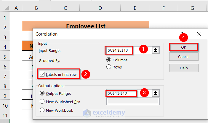
➤ Give the location of the Input Range and Output Range by clicking on the upward arrow > click OK.
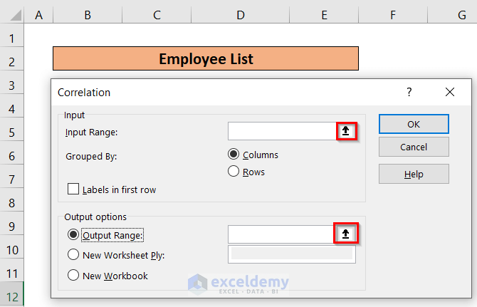
➤ After that, we selected Input Range as $C$4:$E$10 > as our data has a header, we mark on Labels in first row > selected Output Range as $G$4:$I$10 > click OK.
Finally, we can see the correlation coefficients in the following table.
Read More: How to Find Spearman Rank Correlation Coefficient in Excel
Method-3: Using PEARSON Function
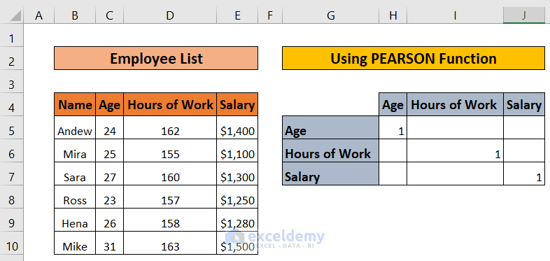
Here, we will use the PEARSON function to calculate the correlation coefficients in the following using the Pearson Function table.
Here, we put value 1 in cells where the two variables are the same.
➤ First of all, we will type the following formula in cell I5 to find out the correlation coefficient between Age and Hours of Work.
=PEARSON(C5:C10,D5:D10)Here,
PEARSON returns Pearson product-moment correlation coefficient that ranges from -1,0 and 1.
The first array is C5:C10, and the 2nd array is D5:D10.
➤ After that, press ENTER.

Now, we can see the result in cell I5.
Here, the correlation coefficient in cell I5 is greater than 0, which indicates a positive correlation.

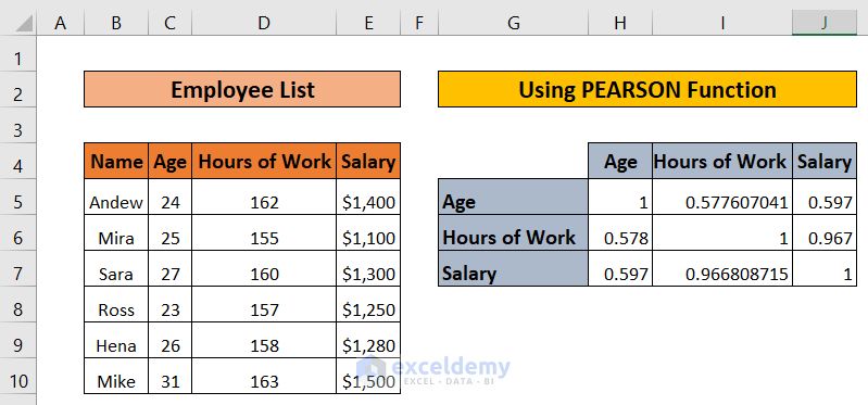
➤ After that, we will use the PEARSON function in other cells as well to calculate correlation coefficients.
Finally, we can see the result in the following using the PEARSON Function table.
Read More: How to Calculate Pearson Correlation Coefficient in Excel
Download Workbook
Conclusion
Here, we tried to show you 3 methods to calculate the correlation coefficient in Excel. Thank you for reading this article, we hope this was helpful. If you have any queries or suggestions, feel free to know us in the comment section.
Correlation Coefficient in Excel: Knowledge Hub
- How to Find Coefficient of Determination in Excel
- How to Calculate Intraclass Correlation Coefficient in Excel
- How to Find Correlation Coefficient in Excel Scatter Plot

